Ocean Carbon & Biogeochemistry
Studying marine ecosystems and biogeochemical cycles in the face of environmental change
  • Home
  • About OCB
    • About Us
    • Scientific Breadth
      • Biological Pump
      • Changing Marine Ecosystems
      • Changing Ocean Chemistry
      • Estuarine and Coastal Carbon Fluxes
      • Ocean Carbon Uptake and Storage
      • Ocean Observatories
    • Code of Conduct
    • Get Involved
    • Project Office
    • Scientific Steering Committee
    • OCB committees
      • Ocean Time-series
      • US Biogeochemical-Argo
      • Ocean-Atmosphere Interaction
  • Activities
    • Summer Workshop
    • OCB Webinars
    • Guidelines for OCB Workshops & Activities
    • Topical Workshops
      • CMIP6 Models Workshop
      • Coastal BGS Obs with Fisheries
      • C-saw extreme events workshop
      • Expansion of BGC-Argo and Profiling Floats
      • Fish, fisheries and carbon
      • Future BioGeoSCAPES program
      • GO-BCG Scoping Workshop
      • Lateral Carbon Flux in Tidal Wetlands
      • Leaky Deltas Workshop – Spring 2025
      • Marine CDR Workshop
      • Ocean Nucleic Acids ‘Omics
      • Pathways Connecting Climate Changes to the Deep Ocean
    • Small Group Activities
      • Aquatic Continuum OCB-NACP Focus Group
      • Arctic-COLORS Data Synthesis
      • BECS Benthic Ecosystem and Carbon Synthesis WG
      • Carbon Isotopes in the Ocean Workshop
      • CMIP6 WG
      • Filling the gaps air–sea carbon fluxes WG
      • Fish Carbon WG
      • Meta-eukomics WG
      • mCDR
      • Metaproteomic Intercomparison
      • Mixotrophs & Mixotrophy WG
      • N-Fixation WG
      • Ocean Carbonate System Intercomparison Forum
      • Ocean Carbon Uptake WG
      • OOI BGC sensor WG
      • Operational Phytoplankton Observations WG
      • Phytoplankton Taxonomy WG
    • Other Workshops
    • Science Planning
      • Coastal CARbon Synthesis (CCARS)
      • North Atlantic-Arctic
    • Ocean Acidification PI Meetings
    • Training Activities
      • PACE Hackweek 2025
      • PACE Hackweek 2024
      • PACE Training Activity 2022
  • Science Support
    • Data management and archival
    • Early Career
    • Funding Sources
    • Jobs & Postdocs
    • Meeting List
    • OCB Topical Websites
      • Ocean Fertilization
      • Trace gases
      • US IIOE-2
    • Outreach & Education
    • Promoting your science
    • Student Opportunities
    • OCB Activity Proposal Solicitations
      • Guidelines for OCB Workshops & Activities
    • Travel Support
  • Publications
    • OCB Workshop Reports
    • Science Planning and Policy
    • Newsletter Archive
  • Science Highlights
  • News

Archive for Clivar Joint Issue – Page 2

Impact of ENSO on biogeochemistry and lower trophic level response in the California Current System

Posted by mmaheigan 
· Thursday, February 16th, 2017 

El Niño events are one of the “most spectacular instances of interannual variability in the ocean” with “profound consequences for climate and the ocean ecosystem” (Cane 1986). Perturbations in the atmosphere directly influence the ocean with long-term effects on environmental variability in the tropical Pacific Ocean as the El Niño-Southern Oscillation (ENSO) shifts between El Niño, neutral, and La Niña states on a timescale of two to seven years. On longer timescales, teleconnections from the tropics to extratropical regions drive Pacific decadal variability, and these can be both oceanic and atmospheric in nature. Mid-latitude variability of the Pacific Decadal Oscillation (PDO) has been associated with ENSO (e.g., Newman et al. 2003) and is distinguished from ENSO in part by its multidecadal timescale (20-30 years; 50 years). The PDO is dependent upon ENSO as a response to the combined effects of atmospheric noise (Newman et al. 2003), as well as the asymmetry of the ENSO cycle (Rodgers et al. 2004). Therefore, when discussing decadal variability of the northeast Pacific, we are referring to the delayed impacts of ENSO.

Ecosystem impacts of northeast Pacific variability

Given the complex influence of tropical climate on northeast Pacific ecosystems, there is significant overlap between ENSO signals and higher frequency modes of the PDO Index. It is widely recognized that interactions between these two climate modes drive substantial ecosystem variability on a range of time and space scales. Large regime shifts in the North Pacific that have reverberated throughout the ecosystem, from physics to fish, are recurring patterns now associated with low-frequency changes in sea surface temperature (SST) that characterize the PDO (e.g., Mantua et al. 1997). Some of the higher-frequency fluctuations in ecosystem variables of the northeast Pacific that have not been successfully attributed to PDO or ENSO are now thought to be driven by an intermediate mode of variability called the North Pacific Gyre Oscillation (NPGO). While the PDO is characterized as the first empirical orthogonal function (EOF) of SST, NPGO is defined as the first EOF of both SST and sea surface height (SSH) anomalies (Di Lorenzo et al. 2008). Compared to PDO and ENSO, NPGO is more closely tied to variations in salinity, nutrient upwelling, and chlorophyll a (chl-a) in the long-running California Cooperative Oceanic Fisheries Investigations (CalCOFI) time-series. DiLorenzo et al. (2008) suggest that major ecosystem regime shifts require a simultaneous and opposite sign reversal of the NPGO and PDO, as was seen shortly after the massive ENSO event of 1997/98, and all three indices relate back to dynamics in the tropical Pacific. The struggle is to understand how these low- to high(er)-frequency modes of variability in the climate and physics drive fluctuations in biogeochemistry and coastal ecology.

As discussed by Jacox et al. (this post), there is an expected or canonical set of physical conditions associated with ENSO in the California Current System (CCS). This physical response to ENSO generally includes: 1) changes in surface wind stress that alter the strength of coastal upwelling and downwelling; 2) remote oceanic forcing by coastally trapped waves that propagate poleward along the US West Coast and modify thermocline depth and coastal stratification; and 3) changes to alongshore advection (Jacox et al., this post). The ecological response of the coastal marine environment includes changes in primary production and the community composition of plankton and higher trophic levels that can be directly or more subtly related to these physical factors. Primary production is driven by vertical nutrient flux to well-lit surface waters; nutrient supply is related to upwelling magnitude, upwelling source depth, and nutrient concentrations at the source depth. ENSO-related processes are also important for interannual and seasonal variability of oxygen concentrations and carbonate biogeochemistry on the Washington and Oregon Shelves (Siedlecki et al. 2015). In this article, we highlight some of the modeling and observational studies that have successfully attributed ENSO-like variability to specific impacts on the biogeochemistry and lower-trophic level organisms of the northeast Pacific and CCS.


Carbon dioxide

Numerical models are widely employed to diagnose climatic forcing of the physical and biogeochemical conditions of the northeast Pacific. For instance, using a fully coupled ocean and biogeochemical model, Xiu and Chai (2014) found that after accounting for atmospheric effects, the air-sea flux and resulting pCO2 of sea water in the Pacific was significantly correlated (0.6) to the Multivariate ENSO Index (MEI) with a lag of ten months. Similarly, Wong et al. (2010) found that sea surface pCO2 was significantly correlated with the MEI in the northeast Pacific. Biogeochemical models of different complexity have also highlighted the connection between PDO and the interannual variability of air-sea CO2 fluxes (e.g., McKinley et al. 2006). These studies also demonstrate that the individual components controlling surface ocean pCO2 in the northeast Pacific respond to PDO with significant amplitudes, but that their combined influence has a relatively small effect on the CO2 fluxes in this region. Xiu and Chai (2014) showed that the dominant driver of North Pacific pCO2 variability is anthropogenic CO2, whereas air-sea CO2 flux is more closely correlated with the PDO and the NPGO.


Nutrients and chlorophyll

In the coastal regions of the northeast Pacific, such as the CCS, ENSO significantly impacts the nutrient supply due to modifications of upwelling and source waters mentioned above (Jacox et al., this post). At the peak of the El Niño season in December-January, Frischknecht et al. (2016) found a pattern in the development of chlorophyll events through a modeling study focused on the CCS. Around the onset of the El Niño year, chlorophyll anomalies were consistently low. This pattern was even more pronounced during the spring of the following year. In spring of the second year (i.e. with the onset of the upwelling season), all events shared the development of a strong negative chlorophyll anomaly. Frischknecht et al. (2016) attributed this phenomenon to a persistent lack of nutrients to support production driven by a combination of physical mechanisms impacting the thermocline (Jacox et al. 2015; 2016; this post) and light limitation at the onset of the upwelling season. Consequently, El Niño events disrupt the biogeochemical cycling in these systems for months, even years, after the event is over. The observations in Oregon, from the Newport line in Fisher et al. (2015), detail the nitrate anomalies from 1995 to 2015, and the nitrate anomalies remain negative long after the Niño-3.4 SST anomaly suggested that the event was over. This may contribute to the success surrounding seasonal forecast systems like J-SCOPE, in which forecasts of biogeochemical parameters (e.g., bottom oxygen) outperformed those of physical variables (e.g., SST) in terms of predictive skill (Siedlecki et al. 2016).

Oxygen and carbon

The relationship between ENSO and nutrient availability from source waters can serve as an analog for oxygen and carbon content. We would expect from observed stoichiometry that when nutrients are low, oxygen is relatively high and carbon is low. In California, this has been documented: El Niño events correlate to higher oxygen and pH, while La Niña events are correlated with lower oxygen and pH (e.g., Nam et al. 2011). In the northern CCS along the Washington and Oregon coasts, the interannual variability in oxygen content of source waters has been correlated to NPGO more than ENSO (Peterson et al. 2013). Consistent with these findings, oxygen has been increasing since 2010 and aragonite saturation state (a measure of the availability of carbonate ion to calcifying organisms) has been elevated in 2015-2016 relative to the year prior in both Oregon and California (McClatchie et al. 2016).


Primary production & particle export

As an eastern boundary upwelling region, the CCS is among the most productive in the world in terms of primary production and fisheries. The suppression of nutrient availability described above can be thought of as reduced “upwelling efficacy” that leads to reduced primary production in the CCS, while La Niña often has the opposite effect due to associated increases in the upwelling efficacy (Jacox et al. 2015). In the southern CCS, the 1997/1998 El Niño led to a significant deepening of the nutricline, with the strongest effects along CalCOFI Line 80, and a pronounced regional reduction of primary production (Bograd and Lynn 2001). The uptake of silicon increased in central California (Santa Barbara Channel) during the onset of the 1997 event, suggesting that diatoms were major drivers of the primary productivity prior to the 1998 spring season when overall productivity was reduced in response to density surface adjustments (Shipe and Brzezinski 2003). Despite reductions in surface layer primary productivity in response to the El Niño, export ratios of particulate organic carbon and particulate organic nitrogen increased during the spring of 1998 relative to the 1994-1997 period, while biogenic Si flux decreased in response to the El Niño (Shipe et al. 2002). This counterintuitive result appears to be due to an increase in particulate material exported to depth. By 1999, ratios of Si/N and Si/C had not recovered to pre-El Nino conditions.


Phytoplankton community composition

Warmer waters and changes in nutrient supply associated with ENSO can lead to phytoplankton community shifts such as an influx of coccolithophores or an increase in harmful algal blooms (HABs). The most common harmful algal bloom organism in the CCS is the diatom genus Pseudo-nitzschia. McCabe et al. (2016) recently observed a link between the Oceanic Niño Index (ONI), the Pseudo-nitzschia growth rate anomaly determined from temperature-growth relationships, and domoic acid levels in razor clams over a 16-year period (Figure 1), implicating El Niño-driven warming in the unprecedented 2015 HAB along the US West Coast. Similarly, McKibben et al. (2017) linked warm phases of the PDO and ONI to domoic acid in shellfish in the northern CCS. The toxic blooms off Newport in 2015 were the most prolonged (late-April through October 2015) and among the most toxic ever observed off Oregon (Du et al. 2015; McKibben et al. 2017). Conversely, Santa Barbara Basin sediment trap data showed no significant correlation between a 15-year record of domoic acid levels and PDO, NPGO, or ENSO indices; however, there was a strong change point in the frequency and toxicity of these blooms following the 1997/1998 ENSO (Sekula-Wood et al. 2011).

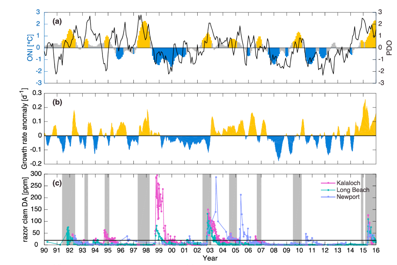
Figure 1. Records of razor clam toxicity and the potential growth rate anomaly for Pseudo-nitzschia spp. are plotted below the Oceanic Niño Index (gold = El Niño, blue = La Niña, gray = neutral) to illustrate the association between ENSO events and harmful algal blooms in the northern CCS. The potential for Pseudo–nitzschia growth does not always coincide with records of high domoic acid in shellfish, e.g., 1997 El Niño. Figure adapted from McCabe et al. (2016).


Zooplankton community composition

Off the Oregon coast, a 21-year time-series of fortnightly hydrography and plankton sampling of shelf and slope waters showed that the water masses (and thus the plankton) that dominate shelf and slope waters vary seasonally, interannually, and on decadal scales. Thus, it is a simple matter to track the timing of summer or winter arrival, ENSO events, and changes in sign of the PDO (Figure 2). During summer months, northerly winds drive surface waters offshore (Ekman transport), which are replaced by the upwelling of cold nutrient-rich waters that penetrate the continental shelf and fuel high primary production. Northerly winds also enhance the southward transport of water (and plankton) from the coastal Gulf of Alaska into the coastal northern CCS, and these species are referred to as ‘cold water’ or ‘northern species.’ During winter, the winds reverse and the poleward Davidson current transports warm coastal water from southern California to the northern CCS, bringing with it ‘southern species’ of plankton. On longer timescales (5-10 years), cold-water, northern copepods are largely replaced by warm-water, southern copepods during El Niño events (Fisher et al. 2015) and during the positive phase of the PDO (Keister et al. 2011). Incorporating the physiological response of these zooplankton groups into biogeochemical-ecosystem models (in addition to the effects of physical transport) will be essential for advancing our predictive capacity of plankton communities in the CCS.

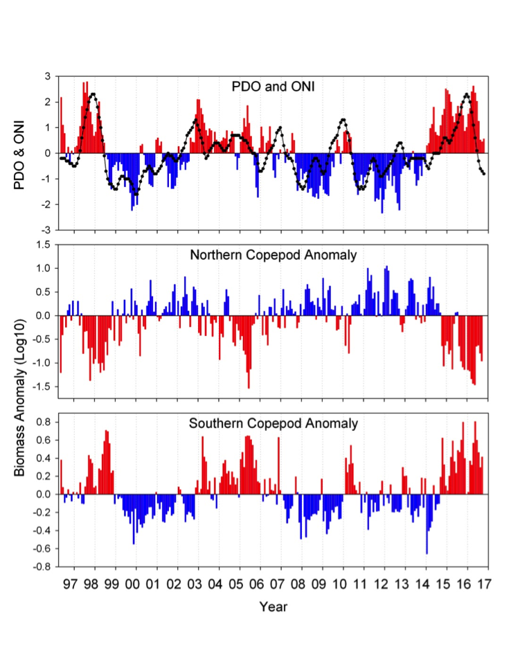
Figure 2. Monthly time series of the Pacific Decadal Oscillation and Oceanic Niño Index (upper) and monthly-averaged biomass anomalies of northern copepods (middle) and southern copepods (lower). Note the high coherence between the PDO and ONI with the copepod time series – positive anomalies of northern copepods are correlated with negative PDO and ONI; positive anomalies of southern copepods are correlated with positive PDO and ONI.


Predicting ecosystem response to ENSO: Now and in the future

State-of-the-art models, in situ measurements, and available satellite observations are all required to adequately characterize short- and long-term physical dynamics associated with ENSO and Pacific decadal variability. Seasonal-to-interannual forecasting of the ecosystem response to ENSO in the CCS and throughout the northeast Pacific will depend on our understanding of how interannual climate variability alters ocean biogeochemistry and productivity at the base of the food web, and therefore how predictive models should be modified to capture the dynamic range introduced by these anomalous events. Unusual warm water anomalies, as observed during large ENSO events, may serve as important analogs for assessing the impacts of long-term warming on the pelagic ecosystem of the CCS. Regional simulations suggest similarities between the physical drivers leading to biogeochemical variability from ENSO and those in projected future upwelling systems (Rykaczewski and Dunne 2010). Further exploration of the mechanisms and predictive skill of forecasts on seasonal timescales will enhance our understanding and improve our projections further into the future. Global climate models are unable to anticipate anomalous warming events such as major ENSO events. As such, they are unable to detect large-scale events related to shifts in the distribution of pelagic species or track ecological changes associated with such events. Furthermore, the evaluation of model-based forecasts and projections of ecosystem variations and changes across timescales requires that long-term physical, biogeochemical, and ecological observation programs are maintained and others initiated. High-resolution modeling approaches for forecasts and projections should also be prioritized, so that ecosystem impacts of future climate anomalies can be anticipated and understood in greater detail.


Authors

Clarissa Anderson (Scripps Institution of Oceanography)
Samantha Siedlecki (University of Washington)
Cecile Rousseaux (NASA Goddard Space Flight Center, Universities Space Research Association)
Brian Powell (University of Hawaii, Manoa)
Bill Peterson (NOAA Northwest Fisheries Science Center)
Chris Edwards (University of California, Santa Cruz)

References

Bograd, S. J., & Lynn, R. J. (2001). Physical‐biological coupling in the California Current during the 1997–99 El Niño‐La Niña Cycle. Geophysical Research Letters, 28(2), 275-278.

Cane, M. A., S. E. Zebiak, and S. C. Dolan, 1986: Experimental forecasts of El Niño. Nature 321, 827–832, doi:10.1038/321827a0.

Di Lorenzo, E., and Coauthors, 2008: North Pacific Gyre Oscillation links ocean climate and ecosystem change. Geophys. Res. Lett., 35, doi:10.1029/2007gl032838.

Du, X., W. Peterson, and L. O’Higgins, 2015: Interannual variations in phytoplankton community structure in the northern California Current during the upwelling seasons of 2001-2010. Mar. Ecol. Prog. Ser., 519, 75-87, doi: 10.3354/meps11097.

Fisher, J. L., W. T. Peterson, and R. Rykaczewski, 2015: The impact of El Niño events on the pelagic food chain in the northern California Current. Global Change Bio., 21, 4401-4414, doi:10.1111/gbc.13054.

Frischknecht, M., M. Münnich, and N. Gruber, 2016: Local atmospheric forcing driving an unexpected California Current System response during the 2015–2016 El Niño, Geophys. Res. Lett., 43, doi:10.1002/2016GL071316.

Jacox, M. G., J. Fiechter, A. M. Moore, and C. A. Edwards, 2015: ENSO and the California Current coastal upwelling response. J. Geophys. Res., 120, 1691–1702, doi: 10.1002/2014JC010650..

Jacox, M., E. L. Hazen, K. D. Zaba, D. L. Rudnick, C. A. Edwards, A. M. Moore, and S. J. Bograd, 2016: Impacts of the 2015–2016 El Niño on the California Current System: Early assessment and comparison to past events. Geophys. Res. Lett. 43, 7072-7080, doi:10.1002/2016GL069716.

Keister, J. E., E. Di Lorenzo, C. A. Morgan, V. Combes, and W. T. Peterson, 2011: Zooplankton species composition is linked to ocean transport in the Northern California Current. Glob. Change Bio., 17, 2498-2511, doi: 10.1111/j.1365-2486.2010.02383.x.

Liu, Z., and M. Alexander, 2007: Atmospheric bridge, oceanic tunnel, and global climatic teleconnections. Rev. Geophy., 45, doi: 10.1029/2005RG000172.

Mantua, N. J., S. R. Hare, Y. Zhang, J. M. Wallace, and R. C. Francis, 1997: A Pacific interdecadal climate oscillation with impacts on salmon production. Bull. Amer. Meteorol. Soc., 78, 1069–1079, doi: 10.1175/1520-0477(1997)078<1069:APICOW>2.0.CO;2.

McCabe, R. M., and Coauthors, 2016: An unprecedented coastwide toxic algal bloom linked to anomalous ocean conditions. Geoph. Res. Lett., 43, doi: 10.1002/2016GL070023.

McClatchie, S., A. R. Thompson, S. R. Alin, S. Siedlecki, W. Watson, and S. J. Bograd, 2016: The influence of Pacific Equatorial Water on fish diversity in the southern California Current System. J. Geophy. Res., 121, 6121-6136, doi: 10.1002/2016JC011672.

McKibben, S. M., W. Peterson, M. Wood, V. L. Trainer, M. Hunter, and A. E. White, 2017: Climatic regulation of the neurotoxin domoic acid. Proc. Nat. Acad. Sci., 114, 239-244, doi: 10.1073/pnas.1606798114.

Mckinley, G.A., and Coauthors, 2006: North Pacific carbon cycle response to climate variability on seasonal to decadal timescales. J. Geophy. Res., 111, doi: 10.1029/2005JC003173.

Nam, S., H. J. Kim, and W. Send, 2011: Amplification of hypoxic and acidic events by La Niña conditions on the continental shelf off California. Geophy. Res. Lett., 38, doi: 10.1029/2011GL049549.

Newman, M., G. P. Compo, and M. A. Alexander, 2003: ENSO-forced variability of the Pacific decadal oscillation. J. Climate, 16, 3853-3857, doi: 10.1175/1520-0442(2003)016<3853:EVOTPD>2.0.CO;2.

Peterson, J. O., C. A. Morgan, W. T. Peterson, and E. Di Lorenzo, 2013: Seasonal and interannual variation in the extent of hypoxia in the northern California Current from 1998–2012. Limnol. Oceanogr., 58, 2279-2292, doi: 10.4319/lo.2013.58.6.2279.

Rodgers, K. B., P. Friederichs, and M. Latif, 2004: Tropical Pacific decadal variability and its relation to decadal modulations of ENSO. J. Climate, 17, 3761-3774, doi: 10.1175/1520-0442(2004)017<3761:TPDVAI>2.0.CO;2.

Rykaczewski, R. R., and J. P. Dunne, 2010: Enhanced nutrient supply to the California Current Ecosystem with global warming and increased stratification in an earth system model. Geophy. Res. Lett., 37, doi: 10.1029/2010GL045019.

Sekula-Wood, E., C. Benitez-Nelson, S. Morton, C. Anderson, C. Burrell, and R. Thunell, 2011: Pseudo-nitzschia and domoic acid fluxes in Santa Barbara Basin (CA) from 1993 to 2008. Harmful Algae, 10, 567–575, doi: 10.1016/j.hal.2011.04.009.

Shipe, R. F., Passow, U., Brzezinski, M. A., Graham, W. M., Pak, D. K., Siegel, D. A., & Alldredge, A. L. (2002). Effects of the 1997–98 El Nino on seasonal variations in suspended and sinking particles in the Santa Barbara basin. Progress in Oceanography, 54(1), 105-127.

Shipe, R. F., and M. A. Brzezinski, 2003: Siliceous plankton dominate primary and new productivity during the onset of El Niño conditions in the Santa Barbara Basin, California. J. Mar. Sys., 42, 127-143, doi: 10.1016/S0924-7963(03)00071-X.

Siedlecki, S. A., N. S. Banas, K. A. Davis, S. Giddings, B. M. Hickey, P. MacCready, T. Connolly, and S. Geier, 2015: Seasonal and interannual oxygen variability on the Washington and Oregon continental shelves. J. Geophy. Res., 120. 608-633, doi: 10.1002/2014JC010254.

Siedlecki, S. A., I. C. Kaplan, A. J. Hermann, T. T. Nguyen, N. A. Bond, J. A. Newton, G. D. Williams, W. T. Peterson, S. R. Alin, and R. A. Feely, 2016: Experiments with seasonal forecasts of ocean conditions for the northern region of the California Current upwelling system. Sci. Rep., 6, 27203, doi: 10.1038/srep27203.

Valsala, V., S. Maksyutov, M. Telszewski, S. Nakaoka, Y. Nojiri, M. Ikeda, and R. Murtugudde, 2012: Climate impacts on the structures of the North Pacific air-sea CO2 flux variability. Biogeosci., 9, 477, doi: 10.5194/bg-9-477-2012.

Xiu, P., and F. Chai, 2014: Variability of oceanic carbon cycle in the North Pacific from seasonal to decadal scales. J. Geophy. Res.,119, 5270-5288, doi: 10.1002/2013JC009505.


Modeling to aid management of marine top predators in a changing climate

Posted by mmaheigan 
· Thursday, February 16th, 2017 

Marine top predators can include species that occupy a high trophic level (e.g., predatory sharks), have few predators (e.g., marine turtles), or can exert top-down control on food webs due to their large energetic demands (e.g., whales). While many species in the open ocean are widely distributed (e.g., Read et al. 2013; Reygondeau et al. 2012), the higher trophic levels are noteworthy as they are also wide-ranging (e.g., tuna (Itoh et al. 2003; Block et al. 2011; Hobday et al. 2015), seabirds (Shaffer et al. 2006), turtles (Shillinger et al. 2008; Briscoe et al. 2016)). These wide-ranging species can serve as ecological linkages within and across ocean basins, through both ontogenetic (larvae to adult) and seasonal migrations (Boustany et al. 2010; Hobday et al. 2015; Briscoe et al. 2016). Many wide-ranging marine animals show site fidelity at particular times during their lives or have relatively small and well-defined areas of critical habitat, which facilitates both exploitation (e.g., Hobday et al. 2015) and protection (e.g., Ban et al. 2014). This fidelity can be related to the temporal and spatial predictability of their physical habitats, as evidenced by predictable seasonal aggregations of high-trophic fishes, birds, turtles, and mammals (Scales et al. 2014), which is aided by sensory capabilities that permit them to locate specific physical and biological features.

These species are also of interest, as they are often charismatic, providing commercial, cultural, or ecological value (e.g., Weng et al. 2015). Top predators in marine ecosystems are supported by the productivity of primary and secondary consumers; thus they integrate a range of processes across these lower levels in the trophic food web. Their relatively long life spans and wide-ranging movements mean that many marine predator populations integrate variability across larger spatial and temporal scales than many lower-trophic-level populations (Shaffer et al. 2006). Top predators also have movement and sensory capabilities that permit active targeting of biophysical features (Scales et al. 2014). These characteristics make assessments of top predator populations particularly valuable for investigations of large-scale ecosystem variability and change.

For example, in the California Current System (CCS), plankton (Fisher et al. 2015; Lluch-Belda et al. 2005) and nekton (Lynn 2003; Phillips et al. 2007; Lluch-Belda et al. 2005) exhibit distributional shifts associated with El Niño-Southern Oscillation (ENSO) events, which are echoed by changes in the distribution of top predators. While the distribution of planktonic organisms is indicative of changes in circulation and habitat suitability, shifts in the distributions of top predators and other nekton are often the result of changes in migration patterns based on the availability of prey. Historical observations of the distributions of top predators indicate that along the West Coast of North America, populations are typically displaced poleward during El Niño events. Also, distributions of species with ranges that are typically offshore (e.g., highly migratory fishes) are contracted towards the West Coast, and the catch-per-unit-effort of tunas and yellowtail are often increased in response to the increased availability to nearshore fishers (Sydeman and Allen 1999; Benson et al. 2002; Henderson et al. 2014). Shifts in species distributions attributed to El Niño are often documented in local newspapers and fishing reports as well as in scientific publications (Lluch-Belda et al. 2005; Cavole et al. 2016). However, many predator populations resident to the CCS (e.g., common murre, Cassin’s auklet, and splitnose rockfishes) exhibit extreme negative productivity anomalies during El Niño (Black et al. 2014), and these events are the most prominent anomalies in time-series spanning multiple decades. Mass strandings of pinnipeds (e.g., sea lions) and die-offs of seabirds have also been associated with El Niño events. These unusual mortality events have been attributed to reduced availability of forage fishes and the exacerbated effects of harmful algal blooms that accompanied past El Niño events (McCabe et al. 2016).

This nearshore compression of viable habitat can also expose these species to a range of relatively concentrated anthropogenic threats, including fishing, oil and gas exploration, transport, and pollution (e.g., Ban et al. 2014). For example, Maxwell et al. (2013) combined electronic tracking from eight top predator species in the CCS with data on 24 anthropogenic stressors to develop a metric of cumulative utilization and impact. The distribution of these stressors and species showed that comprehensive management approaches are required, as no single approach was likely to be successful. Predicting the time-varying distribution and abundance of these and other high-trophic-level species may offer additional management insight, and allow a dynamic approach to management and conservation (e.g., Hobday et al. 2014; Scales et al. 2014; Lewison et al. 2015; Maxwell et al. 2015; Hazen et al. 2016).

Using top predators to monitor ocean changes

There is a suite of tools available for monitoring the response of top predator populations and distributions to variation in environmental conditions. At-sea surveys record the presence and abundance of air-breathing marine predators, such as seabirds, whales, sea turtles, and pinnipeds, which can be reliably sighted at the ocean surface or detected using acoustic methods. Standardized, repeat surveys such as the California Cooperative Oceanic Fisheries Investigations (CalCOFI; Bograd et al. 2003) and NOAA’s Cetacean Ship Surveys (e.g., CalCurCEAS 2014; Rankin et al. 2016) provide longitudinal datasets informative for understanding population trends and regional habitat preferences (Forney et al. 2015; Sydeman et al. 2014). When combined with in situ measurements of physical conditions and prey distributions, survey datasets generate insight into the finer-scale biophysical mechanisms that underlie the dynamics of predator-prey interactions (Benoit-Bird et al. 2013; Embling et al. 2012). Over broader scales, aerial surveys are useful for mapping distributions of air-breathers (Barlow & Forney 2007), and as new technologies become more widely available—such as autonomous underwater vehicles (AUVs), unmanned aerial vehicles (UAVs) (Christiansen et al. 2016; White et al. 2016), and passive acoustics (Morano et al. 2012)—they are increasingly used to survey and study predator populations.

Animal tracking and telemetry allow for remote acquisition of data describing movements and behaviors of marine predators as they move freely through their natural environment. Tracking individuals of known age, sex, body condition, and breeding status has revealed previously cryptic at-sea behaviors (Block et al. 2011; Hazen et al. 2012; Hussey et al. 2015). For example, satellite telemetry has revealed the complexities of ocean-basin scale migrations in several populations (e.g., seabirds (Clay et al. 2016; Shaffer et al. 2006), sea turtles (Briscoe et al. 2016), and pinnipeds (Robinson et al. 2012)). Understanding migratory behaviors improves our knowledge of phenology (timing) and increases chances of detecting climate change responses. Telemetry datasets have also proven particularly powerful in identifying important foraging habitats (e.g., Block et al. 2011; Grecian et al. 2016; Raymond et al. 2015). When linked with measures of body condition or population-level metrics, such as breeding success, tracking datasets provide novel insights into population status and responses to physical variability (e.g., Biuw et al. 2007). Together, these technologies have revolutionized understanding of at-sea habitat use by marine predator populations across the global ocean and hold promise for the use of top predators themselves as monitors of ecosystem change.

Additional statistical tools are necessary to relate predator distribution data to their prey and the environment. Species Distribution Models (SDMs) quantify predator habitat preferences by combining movement or distribution datasets with physical data from in situ measurements, satellite remote sensing, or ocean models (Robinson et al. 2011). A variety of techniques are used for modeling habitat preferences, such as Resource Selection Functions (e.g., generalized linear or additive models), machine learning (e.g., regression or classification trees; Elith & Leathwick 2009), and ensemble predictions from multiple algorithms (Scales et al. 2015). SDMs can enhance the value of tracking data in identifying foraging habitats and provide insight into how predictability in the locations of at-sea habitats links to persistence in the physical environment historically, in real-time, or for future projections (Hobday and Hartmann 2006; Hazen et al. 2013; Becker et al. 2014; Hazen et al. 2016). Individual-based or agent-based models link biological responses to heterogeneity and variability in the physical environment using sets of mechanistic rules that underlie biophysical interactions. To date, individual-based models have been used most extensively for lower trophic-level marine predators, such as small pelagic fish (e.g., Pethybridge et al. 2013), as the mechanisms that link the distributions of these organisms to biophysical conditions are generally better understood than for top predators. However, this approach has distinct advantages for modeling top predator habitat use as it explicitly includes prey-field dynamics, an aspect often missing from SDMs owing to the lack of empirical data describing broad-scale prey distributions. Recent advances using regional ocean models with an individual-based model framework have proven effective in modeling predator habitat selection (e.g., California sea lions (Fiechter et al. 2016)) and hold promise for forecasting top predator distributions in changing oceanic seascapes. In particular, a combination of statistical and mechanistic models can identify non-stationarity in predator-environment relationships and can use energetic and movement rules to incorporate prey into predictive models (Muhling et al. 2016).

Managing for a changing climate

Marine top predators are actively managed in many regions to provide social (e.g., tourism), economic (e.g., harvesting), or ecological benefits (e.g., healthy reefs). Traditional management approaches remain an important tool for managing top predators exploited in marine fisheries and addressing conservation objectives. However, in regions with both short-term and long-term change, static spatial management may not represent the best solution when there are competing goals for ocean use (protection or exploitation), as oceanic habitats are mobile and static protection often requires large areas to cover all of the critical habitat for a particular time period (Hobday et al. 2014; Maxwell et al. 2015). Instead, dynamic spatial management may be a suitable alternative, provided that species movements are predictable and suitable incentives exist (Hobday et al. 2014; Maxwell et al. 2015; Lewison et al. 2015). Several approaches, using data and models described in the previous section, can be used to develop a dynamic management approach in response to variable species distributions, including those based on historical patterns (e.g., past responses to ENSO), real-time, and forecasted prediction of species occurrence. Real-time approaches can use observed data (e.g., satellite data or assimilated ocean model output), while seasonal and decadal approaches require validated models and forecasts of ocean state (Figure 1).

Figure 1. Decisions relevant to fisheries, aquaculture, and conservation sectors at forecasting timescales are noted above the time line. Seasonal forecasting is considered most useful for proactive marine management at this time, with decadal forecasting in its infancy. Modified from Hobday et al. 2016.


The longest standing real-time example comes from the Australian Eastern Tuna and Billfish Fishery (ETBF; Hobday and Hartmann 2006). Fishers in this multi-species longline fishery often target different species—yellowfin, bigeye, and southern bluefin tunas; marlin; and swordfish—depending on seasonal availability and prevailing ocean conditions, and are themselves subjected to management decisions that alter their fishing behavior. In this region, dynamic ocean management was first used in 2003 to reduce unwanted bycatch of quota-limited southern bluefin tuna (SBT). The distribution of likely SBT habitat, which can change rapidly with the movement of the East Australian Current, was used to dynamically regulate fisher access to east coast fishing areas. A habitat preference model was used to provide near real-time advice to management about the likely SBT habitat (Hobday et al. 2010). Managers use these habitat preference reports to frequently update spatial restrictions to fishing grounds, which involve dividing the ocean into a series of zones based on expected distribution of SBT. These restrictions limit unwanted interactions by fishers that do not hold SBT quota (SBT cannot be landed without quota and in that situation must be discarded) and allow access to those that do have SBT quota to operate efficiently (Hobday et al. 2010). The underlying habitat model has evolved from a surface temperature-based model to an integrated surface and sub-surface model, and currently includes a seasonal forecasting element to aid managers and fishers planning for future changes in the location of the habitat zones (Hobday et al. 2011). This ongoing improvement and adaptation of the system has seen new oceanographic products tested and included in the operational model. This dynamic approach has reduced the need for large area closures while still meeting the management goal but does require more flexible fishing strategies to be developed, including planning vessel movements, home port selection, and quota purchase.

In parallel with improved biological data, numerical climate forecast systems have greatly improved over the last 30 years and now have the capability to provide useful seasonal forecasts (National Research Council, 2010). Dynamic forecast systems include i) global climate models (GCMs), which consist of atmosphere, ocean, land, and ice components; ii) observations from multiple sources (e.g., satellites, ships buoys); iii) an assimilation system to merge the observations with the model’s “first guess” to initialize forecasts; and iv) post-processing software to display and disseminate the model output. Such systems are currently used to make forecasts at scales on the order of 100 km on seasonal and even decadal timescales (e.g., Kirtman et al. 2014; Meehl et al. 2014; Stock et al. 2015). In addition, output from the GCMs is being used to drive much higher-resolution forecasts from regional ocean models (Siedlecki et al. 2016). Model skill on seasonal timescales is a function of persistence, multi-year climate modes (e.g., ENSO, IOD), and its teleconnections and transport by ocean currents. Model skill on decadal timescales arises due to anthropogenic climate change and slowly evolving ocean circulation features such as the Atlantic Meridional Overturning Circulation (AMOC; Salinger et al. 2016). GCM-based forecast systems are currently being used to predict sea surface temperature, sub-surface temperatures, and other ocean conditions that are subsequently used in marine resource applications described above (Hobday et al. 2011; Eveson et al. 2015, Figure 2). However, skill from statistical methods is currently on par with those from much more complex and computer-intensive numerical models (Newman 2013; Jacox et al. 2017), and forecast skill will always be limited regardless of the quality of both models and observations due to the chaotic elements of the climate system.

Figure 2. Ecosystem predictions require a suite of inputs and modeling steps to ensure both physical and biological components in the ecosystem are adequately represented. Physical models (from 1 degree to 1/10 degree downscaled models) can be used to predict higher trophic level distributions directly or can be used to drive individual based movement models of prey and predator to incorporate trophic dynamics in ecosystem predictions.


Where do we go from here?

As described above, ocean forecast systems and biological data are being linked to advance top predator management. Three priorities to strengthen this link and better inform management efforts include: (i) gather and share data, (ii) identify effective measures and improve mechanistic understanding of prey availability, and (iii) understand the spatial and temporal overlap between humans and particular focal species.

First, while the capacity to monitor marine top predators has made considerable strides in recent years (Hussey et al. 2015), juvenile portions of many top predator populations can be under-represented and need particular attention (Hazen et al. 2012). Tagging efforts provide detailed data on animal movement and can provide finer-scale data than traditional shipboard surveys. However, there are only a few examples of broad-scale tagging efforts that allow for measurement of diversity and multi-species habitat use, such as the Tagging of Pacific Predators and the Ocean Tracking Network (Block et al. 2011, Hussey et al. 2015). There is a growing trend for these data to be made widely available in repositories (e.g., Ocean Biogeographic Information System Spatial Ecological Analysis of Megavertebrate Populations (OBIS-SEAMAP), Seabird Tracking Database) that allow for greater synthesis than individual datasets alone (Halpin et al. 2006; Lascelles et al. 2016). This should be encouraged as standard practice, as in the oceanographic community (e.g., Global Ocean Ship-Based Hydrographic Investigations Program (GO-SHIP) database). Data collection must continue, as climate variability and change influence the relationship between top predators and their environment, and additional data are necessary to both test and refine predictive models.

Second, while the movements of many highly migratory predators are tied closely to prey availability, most models of marine top predator habitat use remotely sensed or in situ oceanographic measurements as proxies for prey distribution, which is rarely available. The difficulty is in measuring prey distribution at the scales appropriate for predators (e.g., Torres et al. 2008). We can measure fine-scale foraging behavior using archival tag data and associated prey measurements (e.g., Goñi et al. 2009; Hazen et al. 2009), but these ship-based approaches cannot provide data at the scales used in management-focused habitat models (see Lawson et al. 2015). We can model prey distributions mechanistically to inform models of top predator movements (Fiechter et al. 2016), but these approaches have not yet been coupled with real-time prediction. Prey data at migration-wide scales would greatly improve both statistical and mechanistic models by offering insight to where residence times are highest, yet these data remain difficult beyond fine-spatial scales (Benoit-Bird et al. 2013; Boyd et al. 2015).

Finally, both animals and humans use the marine environment at multiple spatial and temporal scales. For example in the Pacific, blue whales migrate from high-latitude foraging grounds to tropical breeding grounds seasonally and travel to discrete foraging hotspots based on prey availability (Bailey et al. 2009), and container vessels are making decisions such as ship speed, choice of shipping lanes, and port of call on multiple time scales as well (Hazen et al. 2016). This requires information on long-term habitat pathways and high-use areas (e.g., for static protection), as well as the shorter-term (e.g., seasonal) triggers of migration and identification of ocean features that result in high prey aggregations and increased residence times. Comparably, a fisher may change her long-term investment decisions (e.g., quota purchase, hiring crew) based on projections of long-term stock dynamics, or may decide when to start fishing seasonally based on weather and proximity to port, or when to set a net based on when fish schools are plentiful (Figure 1). Thus, management approaches could also be nested to include real-time predictions, seasonal forecasts, and decadal projections to inform multiple management processes (Hobday and Hartmann 2006; Hobday et al. 2011; Salinger et al. 2016). This suite of dynamic spatial management tools would represent an adaptive strategy robust to shifting habitats and species in response to climate variability and change.


Authors

Elliott Hazen (NOAA Southwest Fisheries Science Center)
Mike Alexander (NOAA Earth System Research Laboratory)
Steven Bograd (NOAA Southwest Fisheries Science Center)
Alistair J. Hobday (CSIRO, Australia)
Ryan Rykaczewski (University of South Carolina)
Kylie L. Scales (University of the Sunshine Coast, Australia)

References

Ban, N. C., and Coauthors, 2014: Better integration of sectoral planning and management approaches for the interlinked ecology of the open oceans. Mar. Policy, 49, 127-136, doi:10.1016/j.marpol.2013.11.024.

Barlow, J., and K. A. Forney, 2007: Abundance and population density of cetaceans in the California Current ecosystem. Fish. Bull., 105, 509-526.

Becker, E. A., K. A. Forney, D. G. Foley, R. C. Smith, T. J. Moore, and J. Barlow, 2014: Predicting seasonal density patterns of California cetaceans based on habitat models. End. Sp. Res., 23, 1-22, doi:10.3354/esr00548.

Benoit-Bird, K. J., and Coauthors, 2013: Prey patch patterns predict habitat use by top marine predators with diverse foraging strategies. PLoS One, 8, e53348, doi:10.1371/journal.pone.0053348.

Benson, S. R., D. A. Croll, B. Marinovic, F. P. Chavez, and J. T. Harvey, 2002: Changes in the cetacean assemblage of a coastal upwelling ecosystem during El Niño 1997-98 and the La Niña 1999. Prog. Oceanogr., 54, 279-291, doi:10.1016/S0079-6611(02)00054-X.

Biuw, M., and Coauthors, 2007: Variations in behavior and condition of a Southern Ocean top predator in relation to in situ oceanographic conditions. Proc. Nat. Acad. Sci., 104, 13705-13710, doi:10.1073/pnas.0701121104.

Black, B. A., W. J. Sydeman, D. C. Frank, D. Griffin, D. W. Stahle, M. García-Reyes, R. R. Rykaczewski, S. J. Bograd, and W. T. Peterson, 2014: Six centuries of variability and extremes in a coupled marine-terrestrial ecosystem. Science, 345,1498-1502, doi:10.1126/science.1253209.

Block, B. A., and Coauthors, 2011: Tracking apex marine predator movements in a dynamic ocean. Nature, 475, 86-90, doi:10.1038/nature10082.

Bograd, S. J., D. A. Checkley, and W. S. Wooster, 2003: CalCOFI: A half century of physical, chemical, and biological research in the California Current System. Deep Sea Res. II, 50, 2349-2353, doi:10.1016/S0967-0645(03)00122-X.

Boustany, A., R. Matteson, M. R. Castleton, C. J. Farwell, and B. A. Block, 2010: Movements of Pacific bluefin tuna (Thunnus orientalis) in the Eastern North Pacific revealed with archival tags. Prog. Oceanogr., 86, 94-104, doi:10.1016/j.pocean.2010.04.015.

Boyd, C., R. Castillo, G. L. Hunt, A. E. Punt, G. R. VanBlaricom, H. Weimerskirch, and S. Bertrand, 2015: Predictive modelling of habitat selection by marine predators with respect to the abundance and depth distribution of pelagic prey. J. Animal Ecol., 84, 1575-1588, doi:10.1111/1365-2656.12409.

Briscoe, D. K., and Coauthors, 2016: Multi-year tracking reveals extensive pelagic phase of juvenile loggerhead sea turtles in the North Pacific. Movement Ecol., doi:10.1186/s40462-016-0087-4.

Cavole, L. M., and Coauthors, 2016: Biological impacts of the 2013–2015 warm-water anomaly in the Northeast Pacific: Winners, losers, and the future. Oceanogr., 29, 273–285, doi:10.5670/oceanog.2016.32.

Christiansen, F., L. Rojano-Doñate, P. T. Madsen, and L. Bejder, 2016: Noise levels of multi-rotor unmanned aerial vehicles with implications for potential underwater impacts on marine mammals. Front. Mar. Sci., 3, 277, doi:10.3389/fmars.2016.00277.

Clay, T. A., A. Manica, P. G. Ryan, J. R. Silk, J. P. Croxall, L. Ireland, and R. A. Phillips, 2016: Proximate drivers of spatial segregation in non-breeding albatrosses. Sci. Rep., 6, doi:10.1038/srep29932.

Elith, J., and J. R. Leathwick, 2009: Species distribution models: ecological explanation and prediction across space and time. Ann. Rev. Ecol., Evol., Syst., 40, 677-697, doi:10.1146/annurev.ecolsys.110308.120159.

Embling, C. B., J. Illian, E. Armstrong, J. van der Kooij, J. Sharples, K. C. J. Camphuysen, and B. E. Scott, 2012: Investigating fine-scale spatio-temporal predator-prey patterns in dynamic marine ecosystems: a functional data analysis approach. J. App. Ecol., 49, 481-492, doi:10.1111/j.1365-2664.2012.02114.x.

Eveson, J. P., A. J. Hobday, J. R. Hartog, C. M. Spillman, and K. M. Rough, 2015: Seasonal forecasting of tuna habitat in the Great Australian Bight. Fish. Res., 170, 39–49, doi:10.1016/j.fishres.2015.05.008.

Fiechter, J., L. Huckstadt, K. Rose, and D. Costa, 2016: A fully coupled ecosystem model to predict the foraging ecology of apex predators in the California Current. Mar. Ecol. Prog. Ser., 556, 273-285, doi:10.3354/meps11849.

Fisher, J. L., W. T. Peterson, and R. R. Rykaczewski, 2015: The impact of El Niño events on the pelagic food chain in the northern California Current. Glob. Change Biol., 21, 4401–4414, doi:10.1111/gcb.13054.

Forney, K. A., E. A. Becker, D. G. Foley, J. Barlow, and E. M. Oleson, 2015: Habitat-based models of cetacean density and distribution in the central North Pacific. End. Sp. Res., 27, 1-20, doi:10.3354/esr00632.

Grecian, W.J ., and Coauthors, 2016: Seabird diversity hotspot linked to ocean productivity in the Canary Current Large Marine Ecosystem. Biol. Lett., 12, 20160024, doi:10.1098/rsbl.2016.0024.

Goñi, N., I. Arregui, A. Lezama, H. Arrizabalaga, and G. Moreno, 2009: Small scale vertical behaviour of juvenile albacore in relation to their biotic environment in the Bay of Biscay. Tagging and tracking of marine animals with electronic devices. Reviews: Methods and Technologies in Fish Biology and Fisheries, J. Nielsen, J. R. Sibert, A. J. Hobdayet al. Netherlands, Eds., Springer, 9, 51-76, doi:10.1007/978-1-4020-9640-2.

Halpin, P. N., A. J. Read, B. D. Best, K. D. Hyrenbach, E. Fujioka, M. S. Coyne, L. B. Crowder, S. A. Freeman, and C. Spoerri, 2006: OBIS-SEAMAP: developing a biogeographic research data commons for the ecological studies of marine mammals, seabirds, and sea turtles. Mar. Ecol. Prog. Ser., 316, 239-246, doi:10.3354/meps316239.

Haury, L. R., J. A. McGowan, and P. H. Wiebe, 1978: Patterns and processes in the time-space scales of plankton distributions. Patterns in Plankton Communities, J. H. Steele, Ed., Plenum Press, New York, New York, 277-377.

Hazen, E. L., S. M. Maxwell, H. Bailey, S. J. Bograd, M. Hamann, P. Gaspar, B. J. Godley, and G. L. Shillinger, 2012: Ontogeny in marine tagging and tracking science: technologies and data gaps. Mar. Ecol. Prog. Ser., 457, 221-240, doi:10.3354/meps09857.

Hazen, E. L., and Coauthors, 2013: Predicted habitat shifts of Pacific top predators in a changing climate. Nat. Climate Change, 3, 234-238, doi:10.1038/nclimate1686.

Hazen, E. L., and Coauthors, 2016: WhaleWatch: a dynamic management tool for predicting blue whale density in the California. J. App. Ecol., doi: 10.1111/1365-2664.12820.

Henderson, E. E., K. A. Forney, J. P. Barlow, J. A. Hildebrand, A. B. Douglas, J. Calambokidis, and W. S. Sydeman, 2014: Effects of fluctuations in sea-surface temperature on the occurrence of small cetaceans off Southern California. Fish. Bull., 112, 159–177.

Hobday, A. J., and Coauthors, 2014: Dynamic ocean management: Integrating scientific and technological capacity with law, policy and management. Stanford Environ. Law J., 33, 125-165.

Hobday, A. J., K. Evans, J. P. Eveson, J. H. Farley, J. R. Hartog, M. Basson, and T. A. Patterson, 2015: Distribution and migration – Southern bluefin tuna (Thunnus maccoyii). Biology and Ecology of Bluefin Tuna. T. Kitagawa and S. Kimura. London, Eds., CRC Press,189-210, doi:10.1201/b18714-12.

Hobday, A. J., J. Hartog, C. Spillman, and O. Alves, 2011: Seasonal forecasting of tuna habitat for dynamic spatial management. Can. J. Fish. Aq. Sci., 68, 898–911, doi:10.1139/f2011-031.

Hobday, A. J., and K. Hartmann, 2006: Near real-time spatial management based on habitat predictions for a longline bycatch species. Fish. Mgmt. Ecol., 13, 365-380, doi:10.1111/j.1365-2400.2006.00515.x.

Hobday, A. J., J. R. Hartog, T. Timmis, and J. Fielding, 2010: Dynamic spatial zoning to manage southern bluefin tuna capture in a multi-species longline fishery. Fish. Oceanogr., 19(3), 243–253, doi:0.1111/j.1365-2419.2010.00540.x.

Jacox, M. G., M. A. Alexander, C. A. Stock, and G. Hervieux, 2017: On the skill of seasonal sea surface temperature forecasts in the California Current System and its connection to ENSO variability. Climate Dyn., in review.

Hussey, N. E., and Coauthors, 2015: Aquatic animal telemetry: a panoramic window into the underwater world. Science, 348, 1255642, doi:10.1126/science.1255642.

Kirtman, B.P., and Coauthors 2014: The North American Multimodel Ensemble: Phase-1 Seasonal-to-Interannual Prediction; Phase-2 toward Developing Intraseasonal Prediction. Bull. Amer. Meteor. Soc., 95, 585–601, doi:10.1175/BAMS-D-12-00050.1.

Lascelles, B. G., and Coauthors, 2016: Applying global criteria to tracking data to define important areas for marine conservation. Div. Dist., 22, 422-431, doi:10.1111/ddi.12411.

Lawson, G. L., L. A. Hückstädt, A. C. Lavery, F. M. Jaffré, P. H. Wiebe, J. R. Fincke, D. E. Crocker, and D. P. Costa, 2015: Development of an animal-borne “sonar tag” for quantifying prey availability: test deployments on northern elephant seals. Anim. Biotelem., 3, 22, doi:10.1186/s40317-015-0054-7.

Lewison, R. L., and Coauthors, 2015: Dynamic ocean management: Identifying the critical ingredients of dynamic approaches to ocean resource management. Biosci., 65, 486-498, doi:10.1093/biosci/biv018.

Lluch-Belda, D., D. Lluch-Cota, and S. Lluch-Cota, 2005: Changes in marine faunal distributions and ENSO events in the California Current. Fish. Oceanogr., 14, 458–467, doi:10.1111/j.1365-2419.2005.00347.x.

Lynn, R. J., 2003: Variability in the spawning habitat of Pacific sardine (Sardinops sagax) off southern and central California. Fish. Oceanogr., 12, 541–553, doi:10.1046/j.1365-2419.2003.00232.x.

Maxwell, S. M., and Coauthors, 2013: Cumulative human impacts on marine predators. Nat. Comm., 4, 2688, doi:10.1038/ncomms3688.

Maxwell, S. M., and Coauthors, 2015: Dynamic ocean management: Defining and conceptualizing real-time management of the ocean. Mar. Pol., 58, 42–50, doi:10.1016/j.marpol.2015.03.014.

Meehl, G., and Coauthors, 2014: Decadal climate prediction: An update from the trenches. Bull. Amer. Meteor. Soc., 95, 243–267, doi:10.1175/BAMS-D-12-00241.1.

McCabe, R. M., and Coauthors, 2016: An unprecedented coastwide toxic algal bloom linked to anomalous ocean conditions. Geophys. Res. Lett., 43, 10,366–10,376, doi:10.1002/2016GL070023.

Morano, J. L., Rice, A. N., Tielens, J. T., Estabrook, B. J., Murray, A., Roberts, B. L., and Clark, C. W., 2012: Acoustically detected year‐round presence of right whales in an urbanized migration corridor. Con.s Biol., 26, 698-707, doi:10.1111/j.1523-1739.2012.01866.x.

Muhling, B. A., R. Brill, J. T. Lamkin, M. A. Roffer, S. K. Lee, Y. Liu, and F. Muller-Karger, 2016: Projections of future habitat use by Atlantic bluefin tuna: mechanistic vs. correlative distribution models. ICES J. Mar. Sci., doi:10.1093/icesjms/fsw215.

National Research Council, 2010: Assessment of intraseasonal to interannual climate prediction and predictability. Washington, DC: The National Academies Press. doi:10.17226/12878.

Pethybridge, H., D. Roos, V. Loizeau, L. Pecquerie, and C. Bacher, 2013: Responses of European anchovy vital rates and population growth to environmental fluctuations: an individual-based modeling approach. Ecol. Mod., 250, 370-383, doi:10.1016/j.ecolmodel.2012.11.017.

Queiroz, N., N. E. Humphries, G. Mucientes, N. Hammerschlag, F. P. Lima, K. L. Scales, P. I. Miller, L. L. Sousa, R. Seabra, and D. W. Sims, 2016: Ocean-wide tracking of pelagic sharks reveals extent of overlap with longline fishing hotspots. Proc. Nat. Acad. Sci., 113, 1582-1587, doi:10.1073/pnas.1510090113.

Rankin, S., F. Archer, J. L. Keating, J. N. Oswald, M. Oswald, A. Curtis, and J. Barlow, 2016: Acoustic classification of dolphins in the California Current using whistles, echolocation clicks, and burst pulses. Mar. Mamm. Sci., doi:10.1111/mms.12381.

Raymond, B., M. A. Lea, T. Patterson, V. Andrews-Goff, R. Sharples, J. B. Charrassin, M. Cottin, L. Emmerson, N. Gales, R. Gales, and S. D. Goldsworthy, 2015: Important marine habitat off east Antarctica revealed by two decades of multi-species predator tracking. Ecography, 38, 121-129, doi:10.1111/ecog.01021.

Read, B. A., and Coauthors, 2013: Pan genome of the phytoplankton Emiliania underpins its global distribution. Nature, doi:10.1038/nature12221.

Reygondeau, G., O. Maury, G. Beaugrand, J.-M. Fromentin, A. Fonteneau, and P. Cury, 2012: Biogeography of tuna and billfish communities. J. Biogeogr., 39, 114-129, doi:10.1111/j.1365-2699.2011.02582.x.

Robinson, L., J. Elith, A. J. Hobday, R. G. Pearson, B. E. Kendall, H. P. Possingham and A. J. Richardson, 2011: Pushing the limits in marine-based species distribution modelling: lessons from the land present challenges and opportunities. Glob. Ecol. Bio., 20, 789–802, doi:10.1111/j.1466-8238.2010.00636.x.

Robinson, P. W., and Coauthors, 2012: Foraging behavior and success of a mesopelagic predator in the northeast Pacific Ocean: insights from a data-rich species, the northern elephant seal. PLoS One, 7, e36728, doi: 10.1371/journal.pone.0036728.

Salinger, J., and Coauthors, 2016: Decadal-scale forecasting of climate drivers for marine applications. Adv. Mar. Biol. 74: 1-68. doi:10.1016/bs.amb.2016.04.002.

Scales, K. L., P. I. Miller, S. N. Ingram, E. L. Hazen, S. J. Bograd, and R. A. Phillips, 2015: Identifying predictable foraging habitats for a wide-ranging marine predator using ensemble ecological niche models. Div. Dist., 22, 212-224, doi:10.1111/ddi.12389.

Scales, K. L., P. I. Miller, L. A. Hawkes, S. N. Ingram, D. W. Sims and S. C. Votier, 2014: On the Front Line: frontal zones as priority at-sea conservation areas for mobile marine vertebrates. J. App. Ecol., 51, 1575–1583, doi:10.1111/1365-2664.12330.

Shaffer, S. A., and Coauthors 2006: Migratory shearwaters integrate oceanic resources across the Pacific Ocean in an endless summer. Proc. Nat. Acad. Sci., 103, 12799–12802, doi:10.1073/pnas.0603715103.

Shillinger, G. L., and Coauthors, 2008: Persistent leatherback turtle migrations present opportunities for conservation. PLoS Biol., 6, e171. doi:10.1371/journal.pbio.0060171.

Siedlecki, S. A., I. C. Kaplan, A. J. Hermann, T. T. Nguyen, N. A. Bond, J. A. Newton, G. D. Williams, W. T. Peterson, S. R. Alin, and R. A. Feely, 2016: Experiments with seasonal forecasts of ocean conditions for the northern region of the California Current upwelling system. Sci. Rep., 6, 27203, doi:10.1038/srep27203.

Stock, C. A., K. Pegion, G. A. Vecchi, M. A. Alexander, D. Tommasi, N. A. Bond, P. S. Fratantoni, R. G. Gudgel, T. Kristiansen, T. D. O’Brien, Y. Xue and X. Yang X, 2015: Seasonal sea surface temperature anomaly prediction for coastal ecosystems. Prog. Oceanogr., 137, 219-236, doi:10.1016/j.pocean.2015.06.007.

Sydeman, W. J., and S. G. Allen, 1999: Pinniped population dynamics in central California: correlations with sea-surface temperature and upwelling indices. Mar. Mamm. Sci., 15(2), 446-461, doi:10.1111/j.1748-7692.1999.tb00812.x.

Sydeman, W. J., S. A. Thompson, J. A. Santora, J. A. Koslow, R. Goericke, and M. D. Ohman, 2014: Climate-ecosystem change off southern California: time-dependence seabird predator-prey numerical responses. Deep Sea. Res. II, 158–170. doi:10.1016/j.dsr2.2014.03.008.

Weng, K. C., E. Glazier, S. Nicol and A.J. Hobday, 2015: Fishery management, development and food security in the Western and Central Pacific in the context of climate change. Deep Sea Res. II, 113, 301-311, doi:10.1016/j.dsr2.2014.10.025.

White, C. F., Y. Lin, C. M. Clark, and C. G. Lowe, 2016: Human vs robot: Comparing the viability and utility of autonomous underwater vehicles for the acoustic telemetry tracking of marine organisms. J. Exp. Mar. Biol. Ecol., 485, 112-118, doi:10.1016/j.jembe.2016.08.010.

Willis-Norton, E., E. L. Hazen, S. Fossette, G. Shillinger, R. R. Rykaczewski, D. G. Foley, J. P. Dunne, and S. J. Bograd, 2015: Climate change impacts on leatherback turtle pelagic habitat in the Southeast Pacific. Deep Sea Res. II, 113, 260-267, doi:10.1016/j.dsr2.2013.12.019.

Seasonal forecasts of ocean conditions in the California Current Large Marine Ecosystem

Posted by mmaheigan 
· Thursday, February 16th, 2017 

The California Current Large Marine Ecosystem (CCLME) is a productive coastal ecosystem extending from Baja California, Mexico, to British Columbia, Canada. High primary productivity is sustained by inputs of cooler, nutrient-rich waters during seasonal wind-driven upwelling in spring and summer. This high productivity fuels higher trophic levels, including highly valued commercial ($3.5B yr-1) and recreational ($2.5B yr-1) US fisheries (NOAA 2016). The CCLME system experiences large interannual and decadal variability in ocean conditions in response to the El Niño-Southern Oscillation (ENSO) and extratropical climate modes such as the Pacific Decadal Oscillation and the North Pacific Gyre Oscillation (Di Lorenzo et al. 2013). ENSO events affect productivity of the CCLME ecosystem through atmospheric and oceanic pathways. In the former, El Niño triggers a decrease in equatorward winds (Alexander et al. 2002), reducing upwelling and nutrient inputs to coastal surface waters (Schwing et al. 2002; Jacox et al. this issue). In the latter, El Niño events propagate poleward from the equator via coastally trapped Kelvin waves, increasing the depth of the thermocline, and hence decreasing the nutrient concentration of upwelled source waters during El Niño events (Jacox et al. 2015; Jacox et al. this issue). Thus, CCLME productivity, forage fish dynamics, and habitat availability for top predators can vary substantially between years (Chavez et al. 2002; Di Lorenzo et al. 2013; Hazen et al. 2013; Lindegren et al. 2013), and there is increasing recognition of the need to incorporate seasonal forecasts of ocean conditions into management frameworks to improve fisheries management and industry decisions (Hobday et al. 2016; Tommasi et al. 2017a). We describe herein recent improvements in the seasonal prediction of ENSO and how these advances have translated to skillful forecasts of oceanic conditions in the CCLME. We conclude by offering remarks on the implications for ecological forecasting and improved management of living marine resources in the CCLME.

Seasonal ENSO predictions

ENSO is the dominant mode of seasonal climate variability, and while it is a tropical Pacific phenomenon, its effects extend over the entire Pacific basin and even globally. ENSO and its teleconnections influence rainfall, temperature, and extreme events such as flooding, droughts, and tropical cyclones (Zebiak et al. 2015). Because of the extensive societal impacts associated with ENSO, its prediction has been central to the development of today’s state-of–the-art seasonal climate prediction systems. The first attempts at ENSO prediction go back to the 1980s (Cane et al. 1986). Today, resulting from the development of an ENSO observing system located in the equatorial Pacific (McPhaden et al. 1998) and large improvements in our understanding of ENSO dynamics over the last two decades (Neelin et al. 1998; Latif et al. 1998; Chen and Cane 2008), prediction systems can, in general, skillfully predict ENSO up to about six months in advance (Tippett et al. 2012; Ludescher et al. 2014). While such skillful ENSO forecasts may also improve prediction of the extratropical ENSO response, intrinsic variability of the extratropical atmosphere and ocean, and the chaotic nature of weather, will limit extratropical prediction skill no matter how accurately the models—and observations initializing them—predict ENSO itself. ENSO operational forecasts from numerous climate modeling centers are made available in real-time from Columbia University’s International Research Institute for Climate and Society and NOAA’s Climate Prediction Center.

Given its global impact, ENSO provides much of the climate forecasting skill on seasonal timescales (Goddard et al. 2001). While weather is only predictable over a timescale of days (up to about two weeks) owing to the chaotic nature of the atmosphere (Lorenz 1963), predictions of seasonal-scale anomalies are possible because of the ability of global dynamical prediction systems to model atmosphere-ocean coupling processes and other atmosphere forcing factors, such as land and sea ice, which vary more slowly than the atmosphere (Goddard 2001). Low-frequency variations in sea surface temperature (SST), particularly in the tropics, can modulate the atmosphere (as is the case for ENSO), making some weather patterns more likely to occur over the next month or season. Therefore, the ability of the coupled global climate models to skillfully forecast the evolution of observed tropical SSTs, shifts the distribution of likely average weather over the next month or season may be, and allows for skillful prediction of seasonal climate anomalies.

While seasonal predictability is relatively high for SST due to the ocean’s large thermal inertia, assessments of SST predictability have largely been focused on ocean basin-scale modes of variability (e.g., ENSO), linked to regional rainfall and temperature patterns over land. However, recent work has demonstrated that seasonal SST predictions are also skillful in coastal ecosystems (Stock et al. 2015; Hervieux et al. 2017), and, as detailed in the next section, specifically for the CCLME (Jacox et al. 2017).

Seasonal climate predictions in the California Current Large Marine Ecosystem

Recent advances in ENSO prediction and global dynamical seasonal climate prediction systems have enabled skillful seasonal forecasts of SST anomalies in the CCLME after bias correcting the forecasts to remove model drift (Stock et al. 2015; Jacox et al. 2017; Hervieux et al. 2017). Skill of SST anomaly predictions produced by the National Oceanic and Atmospheric Administration (NOAA) North American Multi-Model Ensemble (NMME) is shown in Figure 1. Skill is evaluated through the anomaly correlation coefficient (ACC) between monthly SST anomalies from retrospective forecasts from 1982 to 2009 and observed SST anomalies. Forecasts are skillful (ACC > 0.6) across initialization months for lead times up to about four months (Figure 1). Persistence of the initialized SST anomalies provides much of the prediction skill at these short lead times (Stock et al. 2015; Jacox et al. 2017). Preexisting temperature anomalies at depth may also provide some predictability. Skillful forecasts of February, March, and April SST extend to lead times greater than six months (Figure 1; Stock et al. 2015; Jacox et al. 2017). This ridge of enhanced predictive skill in winter to early spring forecasts is apparent across seasonal forecasting models and arises from the ability of the prediction systems to capture the wintertime coastal signature of predictable basin-scale SST variations (Stock et al. 2015; Jacox et al. 2017). Specifically, the models can skillfully forecast the predictable evolution of meridional winds during ENSO events and the associated changes in upwelling anomalies and SST in the CCLME (Jacox et al. 2017).

Figure 1. Anomaly correlation coefficients (ACCs) as a function of forecast initialization month (x-axis) and lead-time (y-axis) for (left) persistence and (right) NOAA NMME mean for the California Current system (US West Coast, less than 300 km from shore). Note the ridge of high SST anomaly prediction skill exceeding persistence at long lead-times (4-12 months) for late winter-early spring forecasts. Grey dots indicate ACCs significantly above zero at a 5% level; white dots indicate ACCs significantly above persistence at a 5% level. (Adapted from Jacox et al. 2017).


Owing to the severe ecological and economic consequences of extreme SST conditions in the CCLME (e.g., Cavole et al. 2016), it is also instructive to look at forecast performance over time, specifically during the CCLME extreme warm events of 1991-1992, 1997-1998, and 2014-2016, and the CCLME extreme cold events of 1988-1989, 1998-1999, and 2010-2011 (Figure 2). All of the cold events were associated with La Niña conditions, and the first two warm events and 2015-2016 were associated with El Niño. However, the anomalously warm conditions of 2014 and 2015, dubbed “the blob,” were caused by a resilient ridge of high pressure over the North American West Coast that suppressed storm activity and mixing, and allowed a build-up of heat in the upper ocean (Bond et al. 2015).

The forecast system is highly skillful at one-month lead times. It is also skillful at longer lead times of three and six months, as seen by the forecasted February to April SSTs following the 2010-2011 La Niña and the 2015-2016 El Niño (Figure 2). However, at these longer lead times, the forecast system was unable to capture the extreme magnitude of the warm “blob” anomalies during 2014 and 2015 (Figure 2). Also, while fall to winter conditions during the 1991-1992 El Niño and the late winter-early spring conditions following the 1997-1998 El Niño were forecasted with a six-month lead time, the prolonged warm conditions over the 1992 summer and the early transition to anomalously warm conditions during the summer of 1997 were not (Figure 2).

Transitions in and out of the 1991 and 1997 El Niño events were particularly unusual also at the Equator, with El Niño conditions developing late in 1991 and persisting well into the summer of 1992, and El Niño conditions appearing early in summer 1997 (see Figure 2 in Jacox et al. 2015). The spring predictability barrier for ENSO (i.e., a dip in forecast skill for forecasts initialized over the ENSO transition period of March-May; Tippet et al. 2012), as well as weaker teleconnections to the extratropics in summer, may partly explain the lower forecast skill for these El Niño events during summer and fall, and the poorer forecast performance in predicting the early transition to La Niña conditions in 1998-1999 and 2010-2011 (Figure 2).

The forecast system was also unable to predict the cooler conditions over the ENSO-neutral spring and summer of 1991 (Figure 2). The conditional predictability of CCLME winds and SST on ENSO implies that during ENSO-neutral conditions, such as in 1991 and 2014, forecasts of winds are not skillful and SST forecast skill is therefore limited to lead times up to about four months (Jacox et al. 2017). Thus, skillfulness of the seasonal predictions results from a complex interplay of factors that will require further study to identify the underlying mechanisms driving differing levels of robustness.

Figure 2. Predictions at 1-month (red line), 3-month (blue line), and 6-month (green line) lead times of SST anomalies (°C) for the CCLME from the NOAA Geophysical Fluid Dynamics Laboratory (GFDL) CM2.5 FLOR global climate prediction systems and Reynolds OISST.v2 observations (black line) for specific extreme events in the CCLME. Warm events are on the left; cold events are on the right. The dotted lines represent the February to April period of enhanced predictive skill following ENSO events. The x-axis is months since January 1 of the year in which the extreme event started.


Seasonal forecasts for fisheries management applications

While seasonal prediction of living marine resources has been a goal for the past three decades (GLOBEC 1997), operational use of seasonal SST forecasts to inform dynamic management of living marine resources was pioneered in Australia (Hobday et al. 2011), where seasonal SST forecasts are now used to improve the decision making of the aquaculture industry (Spillman and Hobday 2014; Spillman et al. 2015), fishers (Eveson et al. 2015), and fisheries managers (Hobday et al. 2011). Through both increased awareness of climate prediction skill at fishery-relevant scales and of their value to ecosystem-based management, such efforts have now begun to expand to other regions (see Tommasi et al. 2017a, and case studies therein). In the CCLME, recent work has demonstrated that integration of current March SST forecasts into fisheries models can provide useful information for catch limit decisions for the Pacific sardine fishery (i.e., how many sardines can be caught each year?) when combined with existing harvest cutoffs (Tommasi et al., 2017b). Knowledge of future SST conditions can improve predictions of future recruitment and stock biomass and allow for the development of a dynamic management framework, which could increase allowable fisheries harvests during periods of forecasted high productivity and reduce harvests during periods of low productivity (Tommasi et al. 2017b). Hence, integration of skillful seasonal forecasts into management decision strategies may contribute to greater long-term catches than those set by management decisions based solely on either past SST information or on no environmental information at all (Figure3; Tommasi et al., 2017b).

Figure 3. Mean long-term Pacific sardine catch and biomass following catch limit decisions integrating different levels of environmental information. The catch limit incorporating future SST information reflects the uncertainty of a 2-month lead forecast. (Adapted from Tommasi et al. 2017b).


Novel dynamical downscaling experiments in the Northern California Current as part of the JISAO Seasonal Coastal Ocean Prediction of the Ecosystem (J-SCOPE) project (Siedlecki et al. 2016) show that seasonal regional climate forecasts may also be of potential utility for dynamic spatial management strategies in the CCLME (Kaplan et al. 2016). Predictions of ocean conditions from a global dynamical climate prediction system (NOAA NCEP CFS) forced the Regional Ocean Modeling System (ROMS) with biogeochemistry to produce seasonal forecasts of ocean conditions, both at the surface and at depth, with measureable skill up to a four-month lead time (Siedlecki et al. 2016). The downscaling both enables forecasts of fishery-relevant biogeochemical variables such as chlorophyll, oxygen, and pH not yet produced by global forecasting systems, and resolves the fine-scale physical and ecological processes influencing the distribution of managed species within the CCLME. For instance, high-resolution regional implementations of ROMS resolve upwelling and coastal wave dynamics (Jacox et al. 2015; Siedlecki et al. 2016), two processes that drive the CCLME response to ENSO variability, better than coarser-resolution global models. Downscaled forecasts have also driven prototype forecasts of Pacific sardine spatial distribution (Kaplan et al. 2016). Such forecasts have the potential to inform fishing operations, fisheries surveys, and US and Canadian quotas for this internationally shared stock (Kaplan et al. 2016; Siedlecki et al. 2016; Tommasi et al. 2017a).

These CCLME case studies suggest that with recent advancements in state-of-the-art global dynamical prediction systems and regional downscaling models, some skillful seasonal predictions of ocean conditions are possible (Siedlecki et al. 2016; Tommasi et al. 2017a). Seasonal forecast skill may be further improved by improved representation of other features such as ocean eddies and gyre circulations in the extratropics and the basin-wide atmospheric response to SST anomalies in the Kuroshio-Oyashio region (Smirnov et al. 2015). Such skillful seasonal forecasts present opportunities for inclusion in adaptive management strategies for improved living marine resource management and better informed industry operations in the CCLME.


Authors

Desiree Tommasi (Princeton University)
Michael G. Jacox (University of California, Santa Cruz, NOAA Southwest Fisheries Science Center)
Michael A. Alexander Earth System Research Laboratory, NOAA
Francisco E. Werner (NOAA Southwest Fisheries Science Center)
Samantha Siedlecki (University of Washington)
Charles A. Stock Geophysical Fluid Dynamics Laboratory, NOAA
Nicholas A. Bond (University of Washington)

References

Alexander, M. A., I. Bladé, M. Newman, J. R. Lanzante, N. C. Lau, and J. D. Scott, 2002: The atmospheric bridge: The influence of ENSO teleconnections on air-sea interaction over the global oceans. J. Climate, 15, 2205-2231, doi: 10.1175/1520-0442(2002)015<2205:TABTIO>2.0.CO;2.

Bond, N. A., M. F. Cronin, H. Freeland, and N. Mantua, 2015: Causes and impacts of the 2014 warm anomaly in the NE Pacific. Geophys. Res. Lett., 42, 3414–3420, doi:10.1002/2015GL063306.

Cane, M. A., S. E. Zebiak, and S. C. Dolan, 1986: Experimental forecasts of El Niño. Nature 321, 827–832, doi:10.1038/321827a0.

Cavole, L. M., and Coauthors, 2016: Biological impacts of the 2013–2015 warm-water anomaly in the Northeast Pacific: Winners, losers, and the future. Oceanogr., 29, 273–285, doi: 10.5670/oceanog.2016.32.

Chavez, F. P., J. T. Pennington, C. G. Castro, J. P. Ryan, R. P. Michisaki, B. Schlining, P. Walz, K. R. Buck, A. McFadyen, and C. A. Collins, 2002: Biological and chemical consequences of the 1997–1998 El Niño in central California waters. Prog. Oceanogr., 54, 205–232, doi: 10.1016/S0079-6611(02)00050-2.

Chen, D., and M. A. Cane, 2008: El Niño prediction and predictability. J. Comp. Phys., 227, 3625-3640, doi: 10.1016/j.jcp.2007.05.014.

Di Lorenzo, E., and Coauthors, 2013: Synthesis of Pacific Ocean climate and ecosystem dynamics. Oceanogr. 26, 68–81, doi: 10.5670/oceanog.2013.76.

Eveson, J. P., A. J. Hobday, J. R. Hartog, C. M. Spillman, and K. M. Rough, 2015: Seasonal forecasting of tuna habitat in the Great Australian Bight. Fish. Res., 170, 39–49 doi: 10.1016/j.fishres.2015.05.008.

Global Ocean Ecosystem Dynamics (GLOBEC), 1997: Global Ocean Ecosystem Dynamics Science Plan. R. Harris and the members of the GLOBEC Scientific Steering Committee, Eds., IGBP secretariat, Stockholm, Sweden, 83 pp.

Goddard, L., S. J. Mason, S. E. Zebiak, C. F. Ropelewski, R. Basher, and M. A. Cane, 2001: Current approaches to seasonal-to-interannual climate predictions. Int. J. Climatology, 21, 1111–1152, doi: 10.1002/joc.636.

Hazen, E. L., and Coauthors, 2013: Predicted habitat shifts of Pacific top predators in a changing climate. Nat. Climate Change, 3, 234-238, doi:10.1038/nclimate1686.

Hervieux, G., M. Alexander, C. Stock, M. Jacox, K. Pegion, and D. Tommasi, 2017: Seasonal sea surface temperature anomaly prediction skill for coastal ecosystems using the North American multi-model ensemble (NMME). Climate Dyn., submitted.

Hobday, A. J., J. R. Hartog, C. M. Spillman, and O. Alves, 2011: Seasonal forecasting of tuna habitat for dynamic spatial management. Can. J. Fish. Aq. Sci., 68, 898-911, doi: 10.1139/f2011-031.

Hobday, A. J., C. M. Spillman, J. P. Eveson, and J. R. Hartog, 2016: Seasonal forecasting for decision support in marine fisheries and aquaculture. Fish.,. Oceanogr., 25, 45-56, doi: 10.1111/fog.12083.

Jacox, M. G., J. Fiechter, A. M. Moore, and C. A. Edwards, 2015: ENSO and the California Current coastal upwelling response. J. Geophys. Res. Oceans, 120, 1691–1702, doi:10.1002/ 2014JC010650.

Jacox, M., E. L. Hazen, K. D. Zaba, D. L. Rudnick, C. A. Edwards, A. M. Moore, and S. J. Bograd, 2016: Impacts of the 2015–2016 El Niño on the California Current System: Early assessment and comparison to past events. Geophys. Res. Lett. 43, 7072-7080, doi:10.1002/2016GL069716.

Jacox, M. G., M. A. Alexander, C. A. Stock, and G. Hervieux, 2017: On the skill of seasonal sea surface temperature forecasts in the California Current System and its connection to ENSO variability. Climate Dyn., in review.

Kaplan, I. C., G. D. Williams, N. A. Bond, A. J. Hermann, and S. Siedlecki, 2016: Cloudy with a chance of sardines: forecasting sardine distributions using regional climate models. Fish. Oceanogr., 25, 15–27, doi: 10.1111/fog.12131.

Latif, M., A. Sterl, E. Maier-Reimer, and M. M. Junge, 1998: Climate variability in a coupled GCM. Part I: the tropical Pacific. J. Climate, 6, 5–21, doi: 10.1175/1520-0442(1993)006<0005:CVIACG>2.0.CO;2.

Lindegren, M., D. M. Checkley Jr., T. Rouyer, A. D. MacCall, and N. C. Stenseth, 2013: Climate, fishing, and fluctuations of sardine and anchovy in the California Current. Proc. Nat. Acad. Sci., 110, 13672-13677, doi: 10.1073/pnas.1305733110.

Lorenz, E. N. 1963: Deterministic nonperiodic flow. J. Atmos. Sci., 20, 130-141, doi: 10.1175/1520-0469(1963)020<0130:DNF>2.0.CO;2.

Ludescher, J., A. Gozolchiani, M. Bogachev, A. Bunde, S. Havlin, and H. J. Schellnhuber, 2014: Very early warning of next El Niño. Proc. Nat. Acad. Sci., 111, 2064-2066, doi: 10.1073/pnas.1323058111.

McPhaden, M. J., and Coauthors, 1998: The TOGA observing system: a decade of progress. J. Geophys. Res., 103, 14,169-14,240, doi: 10.1029/97JC02906.

Neelin, J. D., D. S. Battisti, A. C. Hirst, F. F. Jin, Y. Wakata, T. Yamagata, and S. E. Zebiak, 1998: ENSO theory. J. Geophys. Res., 103, 14261–14290, doi: 10.1029/97JC03424.

NOAA, 2016: National Marine Fisheries Service Seafood Industry Impacts tool. https://www.st.nmfs.noaa.gov/apex/f?p=160:1.

Schwing, F. B., T. Murphree, L. DeWitt, and P. M. Green, 2002: The evolution of oceanic and atmospheric anomalies in the northeast Pacific during the El Niño and La Niña events of 1995–2001. Prog. Oceanogr., 54, 459–491, doi:10.1016/S0079-6611(02)00064-2.

Siedlecki, S. A., I. C. Kaplan, A. J. Hermann, T. T. Nguyen, N. A. Bond, J. A. Newton, G. D. Williams, W. T. Peterson, S. R. Alin, and R. A. Feely, 2016: Experiments with seasonal forecasts of ocean conditions for the northern region of the California Current upwelling system. Sci. Rep., 6, 27203, doi: 10.1038/srep27203.

Smirnov, D., M. Newman, M. A. Alexander, Y.-O. Kwon, and C. Frankignoul, 2015: Investigating the local atmospheric response to a realistic shift in the Oyashio sea surface temperature front. J. Climate, 28, 1126-1147, doi: 10.1175/JCLI-D-14-00285.1.

Spillman, C. M., J. R. Hartog, A. J. Hobday, and D. Hudson, 2015: Predicting environmental drivers for prawn aquaculture production to aid improved farm management. Aquaculture, 447, 56–65, doi: 10.1016/j.aquaculture.2015.02.008.

Spillman, C. M., and A. J. Hobday, 2014: Dynamical seasonal ocean forecasts to aid salmon farm management in a climate hotspot. Climate Risk Management, 1, 25-38, doi: 10.1016/j.crm.2013.12.001.

Stock, C. A., K. Pegion, G. A. Vecchi, M. A. Alexander, D. Tommasi, N. A. Bond, P. S. Fratantoni, R. G. Gudgel, T. Kristiansen, T. D. O’Brien, Y. Xue, and X. Yang, 2015: Seasonal sea surface temperature anomaly prediction for coastal ecosystems. Prog. Oceanogr., 137, 219-236, doi: 10.1016/j.pocean.2015.06.007.

Tippett, M. K., A. G. Barnston, and S. Li, 2012: Performance of recent multi-model ENSO forecasts. J. App. Meteorol. Climatol., 51, 637–654, doi: 10.1175/JAMC-D-11-093.1.

Tommasi, D., and Coauthors, 2017a. Managing living marine resources in a dynamic environment: the role of seasonal to decadal climate forecasts. Prog. Oceanogr., doi: 10.1016/j.pocean.2016.12.011.

Tommasi, D., C. Stock, K. Pegion, G. A. Vecchi, R. D. Methot, M. Alexander, and D. Checkley, 2017b: Improved management of small pelagic fisheries through seasonal climate prediction. Ecol. App., doi: 10.1002/eap.1458.

Zebiak, S. E., B. Orlove, A. G. Muñoz, C. Vaughan, J. Hansen, T. Troy, M. C. Thomson, A. Lustig, and S. Garvin, 2015: Investigating El Niño-Southern Oscillation and society relationships. WIREs Climate Change, 6, 17–34, doi: 10.1002/wcc.294.


« Previous Page

Filter by Keyword

abundance acidification additionality advection africa air-sea air-sea interactions algae alkalinity allometry ammonium AMO AMOC anoxic Antarctic Antarctica anthro impacts anthropogenic carbon anthropogenic impacts appendicularia aquaculture aquatic continuum aragonite saturation arctic Argo argon arsenic artificial seawater Atlantic atmospheric CO2 atmospheric nitrogen deposition authigenic carbonates autonomous platforms bacteria bathypelagic BATS BCG Argo benthic bgc argo bio-go-ship bio-optical bioavailability biogeochemical cycles biogeochemical models biogeochemistry Biological Essential Ocean Variables biological pump biophysics bloom blue carbon bottom water boundary layer buffer capacity C14 CaCO3 calcification calcite carbon carbon-climate feedback carbon-sulfur coupling carbonate carbonate system carbon budget carbon cycle carbon dioxide carbon export carbon fluxes carbon sequestration carbon storage Caribbean CCA CCS changing marine chemistry changing marine ecosystems changing marine environments changing ocean chemistry chemical oceanographic data chemical speciation chemoautotroph chesapeake bay chl a chlorophyll circulation CO2 coastal and estuarine coastal darkening coastal ocean cobalt Coccolithophores commercial community composition competition conservation cooling effect copepod copepods coral reefs CTD currents cyclone daily cycles data data access data assimilation database data management data product Data standards DCM dead zone decadal trends decomposers decomposition deep convection deep ocean deep sea coral denitrification deoxygenation depth diatoms DIC diel migration diffusion dimethylsulfide dinoflagellate dinoflagellates discrete measurements distribution DOC DOM domoic acid DOP dust DVM ecology economics ecosystem management ecosystems eddy Education EEZ Ekman transport emissions ENSO enzyme equatorial current equatorial regions ESM estuarine and coastal carbon fluxes estuary euphotic zone eutrophication evolution export export fluxes export production extreme events faecal pellets fecal pellets filter feeders filtration rates fire fish Fish carbon fisheries fishing floats fluid dynamics fluorescence food webs forage fish forams freshening freshwater frontal zone functional role future oceans gelatinous zooplankton geochemistry geoengineering geologic time GEOTRACES glaciers gliders global carbon budget global ocean global warming go-ship grazing greenhouse gas greenhouse gases Greenland ground truthing groundwater Gulf of Maine Gulf of Mexico Gulf Stream gyre harmful algal bloom high latitude human food human impact human well-being hurricane hydrogen hydrothermal hypoxia ice age ice cores ice cover industrial onset inland waters in situ inverse circulation ions iron iron fertilization iron limitation isotopes jellies katabatic winds kelvin waves krill kuroshio lab vs field land-ocean continuum larvaceans lateral transport LGM lidar ligands light light attenuation lipids low nutrient machine learning mangroves marine carbon cycle marine heatwave marine particles marine snowfall marshes mCDR mechanisms Mediterranean meltwater mesopelagic mesoscale mesoscale processes metagenome metals methane methods microbes microlayer microorganisms microplankton microscale microzooplankton midwater mitigation mixed layer mixed layers mixing mixotrophs mixotrophy model modeling model validation mode water molecular diffusion MPT MRV multi-decade n2o NAAMES NCP nearshore net community production net primary productivity new ocean state new technology Niskin bottle nitrate nitrogen nitrogen cycle nitrogen fixation nitrous oxide north atlantic north pacific North Sea nuclear war nutricline nutrient budget nutrient cycles nutrient cycling nutrient limitation nutrients OA observations ocean-atmosphere ocean acidification ocean acidification data ocean alkalinity enhancement ocean carbon storage and uptake ocean carbon uptake and storage ocean color ocean modeling ocean observatories ocean warming ODZ oligotrophic omics OMZ open ocean optics organic particles oscillation outwelling overturning circulation oxygen pacific paleoceanography PAR parameter optimization parasite particle flux particles partnerships pCO2 PDO peat pelagic PETM pH phenology phosphate phosphorus photosynthesis physical processes physiology phytoplankton PIC piezophilic piezotolerant plankton POC polar polar regions policy pollutants precipitation predation predator-prey prediction pressure primary productivity Prochlorococcus productivity prokaryotes proteins pteropods pycnocline radioisotopes remineralization remote sensing repeat hydrography residence time resource management respiration resuspension rivers rocky shore Rossby waves Ross Sea ROV salinity salt marsh satellite scale seafloor seagrass sea ice sea level rise seasonal seasonality seasonal patterns seasonal trends sea spray seawater collection seaweed secchi sediments sensors sequestration shelf ocean shelf system shells ship-based observations shorelines siderophore silica silicate silicon cycle sinking sinking particles size SOCCOM soil carbon southern ocean south pacific spatial covariations speciation SST state estimation stoichiometry subduction submesoscale subpolar subtropical sulfate surf surface surface ocean Synechococcus technology teleconnections temperate temperature temporal covariations thermocline thermodynamics thermohaline thorium tidal time-series time of emergence titration top predators total alkalinity trace elements trace metals trait-based transfer efficiency transient features trawling Tris trophic transfer tropical turbulence twilight zone upper ocean upper water column upwelling US CLIVAR validation velocity gradient ventilation vertical flux vertical migration vertical transport warming water clarity water mass water quality waves weathering western boundary currents wetlands winter mixing zooplankton

Copyright © 2025 - OCB Project Office, Woods Hole Oceanographic Institution, 266 Woods Hole Rd, MS #25, Woods Hole, MA 02543 USA Phone: 508-289-2838  •  Fax: 508-457-2193  •  Email: ocb_news@us-ocb.org

link to nsflink to noaalink to WHOI

Funding for the Ocean Carbon & Biogeochemistry Project Office is provided by the National Science Foundation (NSF) and the National Aeronautics and Space Administration (NASA). The OCB Project Office is housed at the Woods Hole Oceanographic Institution.