Ocean Carbon & Biogeochemistry
Studying marine ecosystems and biogeochemical cycles in the face of environmental change
  • Home
  • About OCB
    • About Us
    • Scientific Breadth
      • Biological Pump
      • Changing Marine Ecosystems
      • Changing Ocean Chemistry
      • Estuarine and Coastal Carbon Fluxes
      • Ocean Carbon Uptake and Storage
      • Ocean Observatories
    • Code of Conduct
    • Get Involved
    • Project Office
    • Scientific Steering Committee
    • OCB committees
      • Ocean Time-series
      • US Biogeochemical-Argo
      • Ocean-Atmosphere Interaction
  • Activities
    • Summer Workshop
    • OCB Webinars
    • Guidelines for OCB Workshops & Activities
    • Topical Workshops
      • CMIP6 Models Workshop
      • Coastal BGS Obs with Fisheries
      • C-saw extreme events workshop
      • Expansion of BGC-Argo and Profiling Floats
      • Fish, fisheries and carbon
      • Future BioGeoSCAPES program
      • GO-BCG Scoping Workshop
      • Lateral Carbon Flux in Tidal Wetlands
      • Leaky Deltas Workshop – Spring 2025
      • Marine CDR Workshop
      • Ocean Nucleic Acids ‘Omics
      • Pathways Connecting Climate Changes to the Deep Ocean
    • Small Group Activities
      • Aquatic Continuum OCB-NACP Focus Group
      • Arctic-COLORS Data Synthesis
      • BECS Benthic Ecosystem and Carbon Synthesis WG
      • Carbon Isotopes in the Ocean Workshop
      • CMIP6 WG
      • Filling the gaps air–sea carbon fluxes WG
      • Fish Carbon WG
      • Meta-eukomics WG
      • mCDR
      • Metaproteomic Intercomparison
      • Mixotrophs & Mixotrophy WG
      • N-Fixation WG
      • Ocean Carbonate System Intercomparison Forum
      • Ocean Carbon Uptake WG
      • OOI BGC sensor WG
      • Operational Phytoplankton Observations WG
      • Phytoplankton Taxonomy WG
    • Other Workshops
    • Science Planning
      • Coastal CARbon Synthesis (CCARS)
      • North Atlantic-Arctic
    • Ocean Acidification PI Meetings
    • Training Activities
      • PACE Hackweek 2025
      • PACE Hackweek 2024
      • PACE Training Activity 2022
  • Science Support
    • Data management and archival
    • Early Career
    • Funding Sources
    • Jobs & Postdocs
    • Meeting List
    • OCB Topical Websites
      • Ocean Fertilization
      • Trace gases
      • US IIOE-2
    • Outreach & Education
    • Promoting your science
    • Student Opportunities
    • OCB Activity Proposal Solicitations
      • Guidelines for OCB Workshops & Activities
    • Travel Support
  • Publications
    • OCB Workshop Reports
    • Science Planning and Policy
    • Newsletter Archive
  • Science Highlights
  • News

Archive for model

Identifying the water mass composition of a sample has never been so easy!

Posted by mmaheigan 
· Thursday, August 31st, 2023 

When we collect seawater in any point of the ocean, we are collecting a mix of water masses from different origin that traveled until there keeping their salinity and temperature properties. The Atlantic Ocean is likely the most complex basin in term of water masses containing more than 15 in its depths. Some of them were “born” in the North Atlantic Ocean, others in the Southern Ocean, even in the Mediterranean Sea! And when we collect a seawater sample we can know which water masses are there, where they come from, what happened to each of them during their journey to us, what story can they tell us.

The variation of any non-conservative property (such as dissolved organic carbon or nutrients) in the deep open ocean depends on the mixing of those water masses and on the biogeochemical processes affecting it (such as heterotrophic respiration). But the effect of the water mass mixing is usually very high, so in order to study the biogeochemical processes, it is necessary to remove that effect.

On the other hand, estimating the contribution of the water masses composing a sample is useful to trace the distribution of each water mass identifying the depth of maximum water mass contribution or the depth-range where the water mass is dominant contributing > 50%. Ocean biogeochemists and microbiologists can get more out of their data estimating the impact of water mass mixing on the variability of any chemical (e.g. inorganic nutrients and dissolved organic carbon) or biological (e.g. prokaryotic heterotrophic abundance and production) property.

Knowing the contribution of each water mass to each sample was not an easy task and required expertise on the origin, circulation and mixing patterns of the water masses present in the study area. This could be even harder in very complex oceanic basin such as the deep Atlantic Ocean. The most commonly used methodology is the Optimum Multi-Parameter (OMP) analysis that was first applied by Tomczak in 1981. However, this methodology is time consuming and requires availability of a large set of quality-controlled chemical variables (e.g. nutrients, oxygen,..) together with a deep knowledge of the oceanography of the studied area. Those chemical variables are not always available or do not have the required quality by contrast to potential temperature and salinity that are high standard core variables in any cruise or database. In a recent research article, we applied multi-regression machine learning models to solve ocean water mass mixing. The models tested were trained using the solutions from OMP analyses previously applied to samples from cruises in the Atlantic Ocean. Extremely Randomized Trees algorithm yielded the highest score (R2 = 0.9931; mse = 0.000227). The model allows solving the mixing of water masses in the Atlantic Ocean using potential temperature, salinity, latitude, longitude and depth. Potential temperature and salinity are the most commonly collected and curated variables in oceanography both from oceanographic cruises and autonomous vehicles (e.g. ARGO) avoiding the use of less commonly measured chemical variables which also require longer and time-consuming analyses of both the water samples and the data.

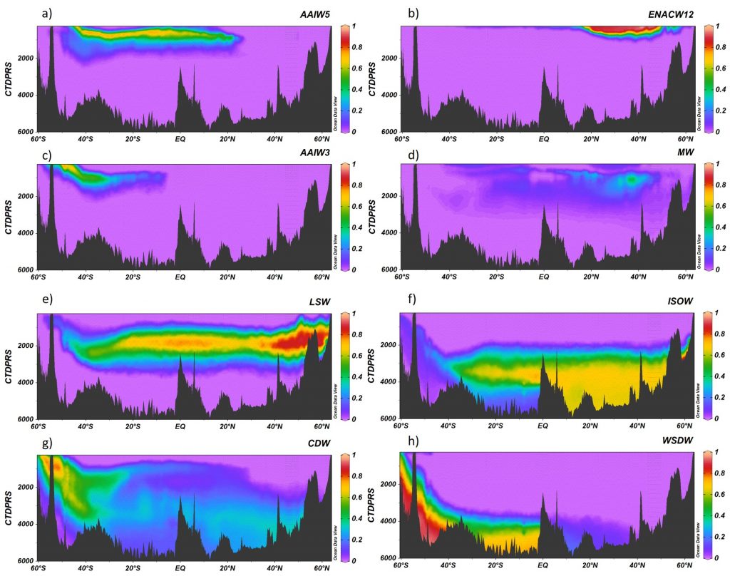
Figure 1. A16 section for the contribution of the water masses (A) AAIW5, (B) ENACW12, (C) AAIW3, (D) MW, (E) LSW, (F) ISOW, (G) CDW and (H) WSDW obtained with the Extremely Randomized Trees algorithm. Ocean Data View software (Schlitzer, 2015).

We also provide the code with instructions where any user can easily introduce the required variables (latitude, longitude, depth, temperature and salinity) of the chosen Atlantic samples and obtain the water mass proportion of each one in a fast and easy way. Actually, it would allow the user to obtain this information in real time during a cruise.

New research using other methods like OMP and its variants can be incorporated to the existing model increasing its accuracy and prediction capacity. Help us to improve the model and increase its spatial resolution!

Ocean biogeochemists and microbiologists can benefit from this tool even if they do not have a deep knowledge of the oceanography of the studied area. Identifying the water masses composition of a sample has never been so easy!

Author
Cristina Romera-Castillo (Instituto de Ciencias del Mar-CSIC, Barcelona, Spain)

Twitter: @crisrcas

Unveiling the Past and Future of Ocean Acidification: A Novel Data Product covering 10 Global Surface OA Indicators

Posted by mmaheigan 
· Wednesday, August 23rd, 2023 

Accurately predicting future ocean acidification (OA) conditions is crucial for advancing research at regional and global scales, and guiding society’s mitigation and adaptation efforts.

As an update to Jiang et al. 2019, this new model-data fusion product:
1. Utilizes an ensemble of 14 distinct Earth System Models from the Coupled Model Intercomparison Project Phase 6 (CMIP6) along with three recent observational ocean carbon data products –>instead of relying on just one model (i.e., the GFDL-ESM2M) this approach reduces potential projection biases in OA indicators.
2. Eliminates model biases using observational data, and model drift with pre-Industrial controls.
3. Covers 10 OA indicators, an expansion from the usual pH, acidity, and buffer capacity.
4. Incorporates the new Shared Socioeconomic Pathways (SSPs).

The use of the most recent observational datasets and a large Earth System Model ensemble is a major step forward in the projection of future surface ocean OA indicators and provides critical information to guide OA mitigation and adaptation efforts.

Figure X. Temporal changes of global average surface ocean OA indicators as reconstructed and projected from 14 CMIP6 Earth System Models after applying adjustments with observational data: (a) fugacity of carbon dioxide (fCO2), (b) total hydrogen ion content ([H+]total), (c) carbonate ion content ([CO32-]), (d) total dissolved inorganic carbon content (DIC), (e) pH on total scale (pHT), (f) aragonite saturation state (Ωarag), (g) total alkalinity content (TA), (h) Revelle Factor (RF), and (i) calcite saturation state (Ωcalc). The asterisk signs on the left-side y-axes show the values in 1750. The numbers along right-side y-axes, i.e., 1-1.9, 1-2.6, 2-4.5, 3-7.0, and 5-8.5, indicate the shared socioeconomic pathway SSP1-1.9, SSP1-2.6, SSP2-4.5, SSP3-7.0, and SSP5-8.5, respectively. These are missing from panel g because the trajectories were more dependent on the model than the SSP.

Authors
Li-Qing Jiang (University Maryland)
John Dunne (NOAA/Geophysical Fluid Dynamics Laboratory)
Brendan R. Carter (University of Washington)
Jerry F. Tjiputra (NORCE Norwegian Research Centre Bjerknes)
Jens Terhaar (Woods Hole Oceanographic Institution)
Jonathan D. Sharp (University of Washington)
Are Olsen (University of Bergen and Bjerknes Centre for Climate Research)
Simone Alin (NOAA/Pacific Marine Environmental Laboratory)
Dorothee C. E. Bakker (University of East Anglia)
Richard A. Feely (NOAA/Pacific Marine Environmental Laboratory)
Jean-Pierre Gattuso (Sorbonne Université)
Patrick Hogan (NOAA/National Centers for Environmental Information)
Tatiana Ilyina (Max Planck Institute for Meteorology)
Nico Lange (GEOMAR Helmholtz Centre for Ocean Research)
Siv K. Lauvset (NORCE Norwegian Research Centre)
Ernie R. Lewis (Brookhaven National Laboratory)
Tomas Lovato (Fondazione Centro Euro-Mediterraneo sui Cambiamenti Climatici)
Julien Palmieri (National Oceanography Centre)
Yeray Santana-Falcón (Université de Toulouse)
Jörg Schwinger (NORCE Norwegian Research Centre)
Roland Séférian (Université de Toulouse)
Gary Strand (US National Center for Atmospheric Research)
Neil Swart (Canadian Centre for Climate Modelling and Analysis)
Toste Tanhua (GEOMAR Helmholtz Centre for Ocean Research)
Hiroyuki Tsujino (JMA Meteorological Research Institute)
Rik Wanninkhof (NOAA/Atlantic Oceanographic Meteorological Laboratory)
Michio Watanabe (Japan Agency for Marine-Earth Science and Technology)
Akitomo Yamamoto (Japan Agency for Marine-Earth Science and Technology)
Tilo Ziehn (CSIRO Oceans and Atmosphere)

Twitter:
@JiangLiqing, @JensTerhaar, @jpGattuso, @j_d_sharp, @AreOlsen, @SimoneAlin, @Dorothee_Bakker, @RFeely, @ilitat, @sivlauvset, @yeraysf, @TosteTanhua,

Filter by Keyword

abundance acidification additionality advection africa air-sea air-sea interactions algae alkalinity allometry ammonium AMO AMOC anoxic Antarctic Antarctica anthro impacts anthropogenic carbon anthropogenic impacts appendicularia aquaculture aquatic continuum aragonite saturation arctic Argo argon arsenic artificial seawater Atlantic atmospheric CO2 atmospheric nitrogen deposition authigenic carbonates autonomous platforms bacteria bathypelagic BATS BCG Argo benthic bgc argo bio-go-ship bio-optical bioavailability biogeochemical cycles biogeochemical models biogeochemistry Biological Essential Ocean Variables biological pump biophysics bloom blue carbon bottom water boundary layer buffer capacity C14 CaCO3 calcification calcite carbon carbon-climate feedback carbon-sulfur coupling carbonate carbonate system carbon budget carbon cycle carbon dioxide carbon export carbon fluxes carbon sequestration carbon storage Caribbean CCA CCS changing marine chemistry changing marine ecosystems changing marine environments changing ocean chemistry chemical oceanographic data chemical speciation chemoautotroph chesapeake bay chl a chlorophyll circulation CO2 coastal and estuarine coastal darkening coastal ocean cobalt Coccolithophores commercial community composition competition conservation cooling effect copepod copepods coral reefs CTD currents cyclone daily cycles data data access data assimilation database data management data product Data standards DCM dead zone decadal trends decomposers decomposition deep convection deep ocean deep sea coral denitrification deoxygenation depth diatoms DIC diel migration diffusion dimethylsulfide dinoflagellate dinoflagellates discrete measurements distribution DOC DOM domoic acid DOP dust DVM ecology economics ecosystem management ecosystems eddy Education EEZ Ekman transport emissions ENSO enzyme equatorial current equatorial regions ESM estuarine and coastal carbon fluxes estuary euphotic zone eutrophication evolution export export fluxes export production extreme events faecal pellets fecal pellets filter feeders filtration rates fire fish Fish carbon fisheries fishing floats fluid dynamics fluorescence food webs forage fish forams freshening freshwater frontal zone functional role future oceans gelatinous zooplankton geochemistry geoengineering geologic time GEOTRACES glaciers gliders global carbon budget global ocean global warming go-ship grazing greenhouse gas greenhouse gases Greenland ground truthing groundwater Gulf of Maine Gulf of Mexico Gulf Stream gyre harmful algal bloom high latitude human food human impact human well-being hurricane hydrogen hydrothermal hypoxia ice age ice cores ice cover industrial onset inland waters in situ inverse circulation ions iron iron fertilization iron limitation isotopes jellies katabatic winds kelvin waves krill kuroshio lab vs field land-ocean continuum larvaceans lateral transport LGM lidar ligands light light attenuation lipids low nutrient machine learning mangroves marine carbon cycle marine heatwave marine particles marine snowfall marshes mCDR mechanisms Mediterranean meltwater mesopelagic mesoscale mesoscale processes metagenome metals methane methods microbes microlayer microorganisms microplankton microscale microzooplankton midwater mitigation mixed layer mixed layers mixing mixotrophs mixotrophy model modeling model validation mode water molecular diffusion MPT MRV multi-decade n2o NAAMES NCP nearshore net community production net primary productivity new ocean state new technology Niskin bottle nitrate nitrogen nitrogen cycle nitrogen fixation nitrous oxide north atlantic north pacific North Sea nuclear war nutricline nutrient budget nutrient cycles nutrient cycling nutrient limitation nutrients OA observations ocean-atmosphere ocean acidification ocean acidification data ocean alkalinity enhancement ocean carbon storage and uptake ocean carbon uptake and storage ocean color ocean modeling ocean observatories ocean warming ODZ oligotrophic omics OMZ open ocean optics organic particles oscillation outwelling overturning circulation oxygen pacific paleoceanography PAR parameter optimization parasite particle flux particles partnerships pCO2 PDO peat pelagic PETM pH phenology phosphate phosphorus photosynthesis physical processes physiology phytoplankton PIC piezophilic piezotolerant plankton POC polar polar regions policy pollutants precipitation predation predator-prey prediction pressure primary productivity Prochlorococcus productivity prokaryotes proteins pteropods pycnocline radioisotopes remineralization remote sensing repeat hydrography residence time resource management respiration resuspension rivers rocky shore Rossby waves Ross Sea ROV salinity salt marsh satellite scale seafloor seagrass sea ice sea level rise seasonal seasonality seasonal patterns seasonal trends sea spray seawater collection seaweed secchi sediments sensors sequestration shelf ocean shelf system shells ship-based observations shorelines siderophore silica silicate silicon cycle sinking sinking particles size SOCCOM soil carbon southern ocean south pacific spatial covariations speciation SST state estimation stoichiometry subduction submesoscale subpolar subtropical sulfate surf surface surface ocean Synechococcus technology teleconnections temperate temperature temporal covariations thermocline thermodynamics thermohaline thorium tidal time-series time of emergence titration top predators total alkalinity trace elements trace metals trait-based transfer efficiency transient features trawling Tris trophic transfer tropical turbulence twilight zone upper ocean upper water column upwelling US CLIVAR validation velocity gradient ventilation vertical flux vertical migration vertical transport warming water clarity water mass water quality waves weathering western boundary currents wetlands winter mixing zooplankton

Copyright © 2025 - OCB Project Office, Woods Hole Oceanographic Institution, 266 Woods Hole Rd, MS #25, Woods Hole, MA 02543 USA Phone: 508-289-2838  •  Fax: 508-457-2193  •  Email: ocb_news@us-ocb.org

link to nsflink to noaalink to WHOI

Funding for the Ocean Carbon & Biogeochemistry Project Office is provided by the National Science Foundation (NSF) and the National Aeronautics and Space Administration (NASA). The OCB Project Office is housed at the Woods Hole Oceanographic Institution.