Ocean Carbon & Biogeochemistry
Studying marine ecosystems and biogeochemical cycles in the face of environmental change
  • Home
  • About OCB
    • About Us
    • Scientific Breadth
      • Biological Pump
      • Changing Marine Ecosystems
      • Changing Ocean Chemistry
      • Estuarine and Coastal Carbon Fluxes
      • Ocean Carbon Uptake and Storage
      • Ocean Observatories
    • Code of Conduct
    • Get Involved
    • Project Office
    • Scientific Steering Committee
    • OCB committees
      • Ocean Time-series
      • US Biogeochemical-Argo
      • Ocean-Atmosphere Interaction
  • Activities
    • Summer Workshop
    • OCB Webinars
    • Guidelines for OCB Workshops & Activities
    • Topical Workshops
      • CMIP6 Models Workshop
      • Coastal BGS Obs with Fisheries
      • C-saw extreme events workshop
      • Ecological Forecasting – North American Coastlines
      • Expansion of BGC-Argo and Profiling Floats
      • Fish, fisheries and carbon
      • Future BioGeoSCAPES program
      • GO-BCG Scoping Workshop
      • Lateral Carbon Flux in Tidal Wetlands
      • Marine CDR Workshop
      • Ocean Nucleic Acids ‘Omics
      • Ocean-Atmosphere Interactions
      • Oceanic Methane & Nitrous Oxide
    • Small Group Activities
      • Aquatic Continuum OCB-NACP Focus Group
      • Arctic-COLORS Data Synthesis
      • BECS Benthic Ecosystem and Carbon Synthesis WG
      • Carbon Isotopes in the Ocean Workshop
      • CMIP6 WG
      • Filling the gaps air–sea carbon fluxes WG
      • Fish Carbon WG
        • Fish Carbon WG Workshop
        • Fish carbon workshop summary
      • Marine carbon dioxide removal
      • Metaproteomic Intercomparison
      • Mixotrophs & Mixotrophy WG
      • N-Fixation WG
      • Ocean Carbonate System Intercomparison Forum
      • Ocean Carbon Uptake WG
      • OOI BGC sensor WG
      • Operational Phytoplankton Observations WG
      • Phytoplankton Taxonomy WG
    • Other Workshops
    • Science Planning
      • Coastal CARbon Synthesis (CCARS)
      • North Atlantic-Arctic
    • Ocean Acidification PI Meetings
    • Training Activities
      • PACE Training Activity
  • Science Support
    • Data management and archival
    • Early Career
    • Funding Sources
    • Jobs & Postdocs
    • Meeting List
    • OCB Topical Websites
      • Ocean Fertilization
      • Trace gases
      • US IIOE-2
    • Outreach & Education
    • Promoting your science
    • Student Opportunities
    • OCB Activity Proposal Solicitations
      • Guidelines for OCB Workshops & Activities
    • Travel Support
  • Publications
    • Ocean Carbon Exchange
    • OCB Workshop Reports
    • Science Planning and Policy
    • Newsletter Archive
  • OCB Science Highlights
  • News

Archive for CCS

Multiyear predictions of ocean acidification in the California Current System

Posted by mmaheigan 
· Thursday, August 20th, 2020 

The California Current System is a highly productive coastal upwelling region that supports commercial fisheries valued at $6 billion/year. These fisheries are supported by upwelled waters, which are rich in nutrients and serve as a natural fertilizer for phytoplankton. Due to remineralization of organic matter at depth, these upwelled waters also contain large amounts of dissolved inorganic carbon, causing local conditions to be more acidic than the open ocean. This natural acidity, compounded by the dissolution of anthropogenic CO2 into coastal waters, creates corrosive conditions for shell-forming organisms, including commercial fishery species.

A recent study in Nature Communications showcases the potential for climate models to skillfully predict variations in surface pH—thus ocean acidification—in the California Current System. The authors evaluate retrospective predictions of ocean acidity made by a global Earth System Model set up similarly to a weather forecasting system. The forecasting system can already predict variations in observed surface pH fourteen months in advance, but has the potential to predict surface pH up to five years in advance with better initializations of dissolved inorganic carbon (Figure 1). Skillful predictions are mostly driven by the model’s initialization and subsequent transport of dissolved inorganic carbon throughout the North Pacific basin.

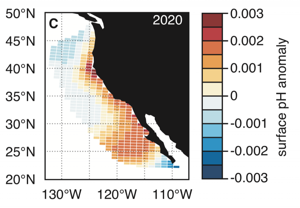
Figure 1. Forecast of annual surface pH anomalies in the California Current Large Marine Ecosystem for 2020. Red colors denote anomalously basic conditions for the given location and blue colors indicate anomalously acidic conditions.

These results demonstrate, for the first time, the feasibility of using climate models to make multiyear predictions of surface pH in the California Current. Output from this global prediction system could serve as boundary conditions for high-resolution models of the California Current to improve prediction time scale and ultimately help inform management decisions for vulnerable and valuable shellfisheries.


Authors:
Riley X. Brady (University of Colorado Boulder)
Nicole S. Lovenduski (University of Colorado Boulder)
Stephen G. Yeager (National Center for Atmospheric Research)
Matthew C. Long (National Center for Atmospheric Research)
Keith Lindsay (National Center for Atmospheric Research)

Elusive protists transport large quantities of silica into the ocean interior

Posted by hbenway 
· Friday, September 7th, 2018 

Phaeodaria are single-celled eukaryotes (a.k.a. protists) belonging to the supergroup Rhizaria. Like diatoms, phaeodarians build up skeletons made of opaline silica, but unlike their emblematic relatives, phaeodarians have been largely ignored in the marine silica cycle.

The contribution of phaeodarians to total biogenic silica (bSiO2) export is markedly enhanced at low total bSiO2 export (analysis did not include data from 2014 due to abnormally depleted phaeodarian population).

In a recent study published in Global Biogeochemical Cycles (also see related Research Spotlight in AGU Eos), authors used a combination of extensive sediment trap deployments and in situ imagery during four cruises of the California Current Ecosystem Long-Term Ecological Research (CCE-LTER) Program off the coast of California to quantify biogenic silica export mediated by giant phaeodarians (>600 µm). These data revealed that giant phaeodarians possess among the highest recorded cellular silica content (up to 43 µg Si cell-1). In addition, measurements of vertical fluxes suggest that these organisms can play a surprisingly large role in silica export (ranging from 10-80% of total silica export) in more oligotrophic waters. Also, because they are most abundant in waters below the euphotic zone, phaeodarians contribute to increased biogenic silica flux in the mesopelagic, in contrast with typically observed decreases in carbon flux with depth. Given their significant contribution to silica export, phaeodarians should be considered in global budgets and models of ocean silica cycles, especially in oligotrophic waters.

Authors
Tristan Biard (Scripps Institution of Oceanography)
Jeffrey W. Krause (University of Southern Alabama)
Michael R. Stukel (Florida State University)
Mark D. Ohman (Scripps Institution of Oceanography)

Untangling the mystery of domoic acid events: A climate-scale perspective

Posted by mmaheigan 
· Thursday, August 3rd, 2017 

The diatom Pseudo-nitzchia produces a neurotoxin called domoic acid, which in high concentrations affects wildlife ranging from mussels and crabs to seabirds and sea lions, as well as humans. In humans, the effects of domoic acid poisoning can range from gastrointestinal distress to memory loss, and even death. Despite being studied in laboratories since the late 1980s, there is no consensus on the environmental conditions that lead to domoic acid events. These events are most frequent and impactful in eastern boundary current regions such as the California Current System, which is bordered by Washington, Oregon, and California. In Oregon alone, there have been six major domoic acid events: 1996, 1998-1999, 2001, 2002-2006, 2010, 2014-2015. McKibben et al. (2017) investigated the regulation of domoic acid at a climate scale to develop and test an applied risk model for the US West Coast” to read “McKibben et al. (2017) investigated the regulation of domoic acid at regional and decadal scales in order to develop and test an applied risk model for the impact of climate on the US West Coast. They used the PDO and ONI climate variability indices, averages of monthly and 3 month running means of SST anomaly values and variability to look at basin-scale ocean conditions. At a local scale, data were from zooplankton sampling every two to four weeks between 1996 to 2015 at hydrographic station offshore of Newport, OR. Additionally, the NOAA NCDC product “Daily Optimum Interpolation, Advanced Very High Resolution Radiometer Only, Version 2, Final+Preliminary SST” was used to obtain the monthly SST anomaly metric, based on combined in situ and satellite data.


(A) Warm and cool ocean regimes, (B) local SST anomaly, and (C and D) biological response. (A) PDO (red or blue vertical bars) and ONI (black line) indices; strong (S) to moderate (M) El Nino (+1) and La Nina (−1) events are labeled. (B) SST anomaly 20 nm off central OR. (C) The CSR anomaly 5 nm off central OR. (D) Monthly OR coastal maximum DA levels in razor clams (vertical bars); horizontal black line is the 20-ppm closure threshold. Black line in D shows the spring biological transition date (right y axis). At the top of the figure, black boxes indicate the duration of upwelling season each year; red vertical bars indicate the timing of annual DA maxima in relationship to upwelling. Gray shaded regions are warm regimes based on the PDO. Dashed vertical lines indicate onset of the six major DA events. The September 2014 arrival of the NE Pacific Warm Anomaly (colloquially termed “The Blob”) to the OR coastal region is labeled on B. “X” symbols along the x axes indicate that no data were available for that month (B–D).

Their findings show that these events have occurred when there is advection of warmer water masses onto the continental shelf from southern or offshore areas. When the warm phase of the Pacific Decadal Oscillation (PDO) and El Niño coincide, the effect is additive. In the warm regime years, there is a later spring biological transition date, weaker alongshore currents, elevated water temperatures, and plankton communities are dominated by subtropical rather than subarctic species. The authors also note relative differences between the prevalence and phenology of domoic acid events in OR, CA and WA, which warrants further study via regional-scale modeling. Overall, this research shows a clear and enhanced risk of toxicity in shellfish during warm phases of natural climate oscillations. If predictions of more extreme warming come to bear, this would potentially lead to increased DA event intensity and frequency in coastal zones around the globe. This will not only affect wildlife, but may cause significant closures of economically important fisheries (e.g., Dungeness crab, anchovy, mussel, and razor clam), which would impact local communities and native populations.


Authors:
Morgaine McKibben (Oregon State Univ., NOAA Northwest Fisheries Science Center)
William Peterson (NOAA Northwest Fisheries Science Center)
Michelle Wood (Univ. Oregon)
Vera L. Trainer (NOAA Northwest Fisheries Science Center)
Matthew Hunter (Oregon Dept. Fish & Wildlife)
Angelicque E. White (Oregon State Univ.)

ENSO impacts on ecosystem indicators in the California Current System

Posted by mmaheigan 
· Thursday, February 16th, 2017 

El Niño-Southern Oscillation (ENSO) events activate long-distance teleconnections through the atmosphere and ocean that can dramatically impact marine ecosystems along the West Coast of North America, affecting diverse organisms ranging from plankton to exploitable and protected species. Such ENSO-related changes to marine ecosystems can ultimately affect humans in many ways, including via depressed plankton and fish production, dramatic range shifts for many protected and exploited species, inaccessibility of traditionally fished resources, more prevalent harmful algal blooms, altered oxygen and pH of waters used in mariculture, and proliferation of pathogens. The principal objective of the Forecasting ENSO Impacts on Marine Ecosystems of the US West Coast workshop was to develop a scientific framework for building an ENSO-related forecast system of ecosystem indicators along the West Coast of North America, including major biological and biogeochemical responses. Attendees realized that a quantitative, biologically-focused forecast system is a much more challenging objective than forecasting the physical system alone; it requires an understanding of the ocean-atmospheric physical system and of diverse organism-level, population-level, and geochemical responses that, in aggregate, lead to altered ecosystem states.

In the tropical ocean, important advances have been made in developing both intensive observational infrastructure (Global Tropical Moored Buoy Array) and diverse dynamical and statistical models that utilize these data in ENSO forecasting. These forecasts are made widely available (e.g., NOAA’s Climate Prediction Center). The most sophisticated ENSO-forecasting efforts use global, coupled ocean-atmosphere climate models that extend ENSO-forecasting skill into seasonal climate forecasting skill for other regions, including the California Current System (CCS). However, both these measurement systems and forecast models are restricted to the physical dynamics of ENSO, rather than biotic and biogeochemical consequences.

Primary modes of influence of El Niño on marine organisms

In this brief discussion, we focus primarily on the warm (El Niño) phases of ENSO, which can have large and generally negative ecosystem consequences, although changes accompanying the cold phases (La Niña) can also be significant. We primarily address pelagic ocean processes, which merely reflect the expertise of the participants at the workshop. Physical mechanisms by which ENSO impacts the U.S. West Coast are more completely explained in Jacox et al. (this issue).

El Niño affects organisms and biogeochemistry via both local and advective processes (Figure 1). ENSO-related changes in the tropics can affect the CCS through an atmospheric teleconnection (Alexander et al. 2002) to alter local winds and surface heat fluxes, and through upper ocean processes (thermocline and sea level displacements and geostrophic currents) forced remotely by poleward propagating coastally trapped waves (CTWs) of tropical origin (Enfield and Allen 1980; Frischkencht et al. 2015; Figure 1). It is important to recognize that ecosystem effects will occur through three primary mechanisms: (1) via the direct action of altered properties like temperature, dissolved O2, and pH on the physiology and growth of marine organisms; (2) through food web effects as changes in successive trophic levels affect their predators (bottom up) or prey (top down); and (3) through changes in advection related to the combination of locally forced Ekman transport and remotely forced geostrophic currents, typically involving poleward and/or onshore transport of organisms. Advective effects can be pronounced, transporting exotic organisms into new regions and altering the food web if these imported species have significant impacts as predators, prey, competitors, parasites, or pathogens.

Figure 1. Schematic illustration of dominant mechanisms through which ENSO impacts biological and biogeochemical processes in the California Current System. Processes include both local effects (e.g., heat budget, winds) and advective effects. Such processes can influence organisms via: (1) (yellow arrow) direct physiological responses to changes in temperature, O2, pH, etc.; (2) (orange arrows) effects that propagate through the food web, as successive trophic levels affect their predators (bottom up, upward-facing orange arrows) or prey (top down, downward-facing orange arrows); (3) (blue arrows) direct transport effects of advection. Top predators are not included here. CTW indicates coastally trapped waves.


I. Poleward and onshore transport

Active, mobile marine fishes, seabirds, reptiles, and mammals may move into new (or away from old) habitats in the CCS as ENSO-related changes occur in the water column and render the physical-chemical characteristics and prey fields more (or less) suitable for them. Planktonic organisms are often critical prey and are, by definition, subject to geographic displacements as a consequence of altered ocean circulation that accompanies El Niño events. Most commonly, lower latitude organisms are transported poleward to higher latitudes in either surface flows or in an intensified California Undercurrent (Lynn and Bograd 2002). However, some El Niño events are accompanied by onshore flows (Simpson 1984), potentially displacing offshore organisms toward shore (Keister et al. 2005).

Two of the most celebrated examples of poleward transport come from distributions of pelagic red crabs (Pleuroncodes planipes) and the subtropical euphausiid (or krill, Nyctiphanes simplex), both of which have their primary breeding populations in waters off Baja California, Mexico (Boyd 1967; Brinton et al. 1999). Pelagic red crabs were displaced approximately 10° of latitude, from near Bahia Magdalena, Baja California, northward to Monterey, California (Glynn 1961; Longhurst 1967) during the El Niño of 1958-1959. This early event was particularly well documented because of the broad latitudinal coverage of the California Cooperative Oceanic Fisheries Investigations (CalCOFI) cruises at the time. Such El Niño-related northward displacements have been documented repeatedly over the past six decades (McClatchie et al. 2016), partly because the red crabs often strand in large windrows on beaches and are conspicuous to the general public. The normal range of the euphausiid Nyctiphanes simplex is centered at 25-30°N (Brinton et al. 1999). N. simplex has been repeatedly detected far to the north of this range during El Niño, extending at least to Cape Mendocino (40.4°N) in 1958 (Brinton 1960), to northern Oregon (46.0°N) in 1983 (Brodeur 1986), and to Newport, Oregon (44.6°N; Keister et al. 2005) and northwest Vancouver Island (50.7°N; Mackas and Galbraith 2002) in 1998. In spring of 2016, N. simplex were extremely abundant in the southern California region (M. Ohman and L. Sala, personal communication) and detected as far north as Trinidad Head (41.0°N) but not in Newport, Oregon (W. Peterson, personal communication). Sometimes such El Niño-related occurrences of subtropical species are accompanied by declines in more boreal species (e.g., Mackas and Galbraith 2002; Peterson et al. 2002), although this is not always the case.

Among the organisms displaced during El Niños, the consequences of transport of predators are poorly understood but likely significant in altering the food web.  Subtropical fishes can be anomalously abundant in higher latitudes during El Niño (Hubbs 1948; Lluch-Belda et al. 2005; Pearcy and Schoener 1987; Pearcy 2002; Brodeur et al. 2006), with significant consequences for the resident food web via selective predation on prey populations.

II. Habitat compression

Many species are confined to a specific habitat that may compress during El Niño. This phenomenon has been observed repeatedly for species and processes related to coastal upwelling in the CCS. During major El Niño events, as the offshore extent of upwelled waters is reduced and becomes confined close to the coast, the zone of elevated phytoplankton (observed as Chl-a) compresses markedly to a narrow zone along the coastal boundary (e.g., Kahru and Mitchell 2000; Chavez et al. 2002). For example, during the strong El Niño spring of 1983, the temperate euphausiid Euphausia pacifica was present in low densities throughout Central and Southern California waters, but 99% of the biomass was unusually concentrated at a single location (station 80.51) very close to Point Conception, where upwelling was still pronounced (E. Brinton, personal communication). The spawning habitat of the Pacific sardine (Sardinops sagax) was narrowly restricted to the coastal boundary during El Niño 1998, but one year later during La Niña 1999, the spawning habitat extended a few hundred kilometers farther offshore (Lo et al. 2005). Market squid, Doryteuthis opalescens, show dramatically lower catches during El Niño years (Reiss et al. 2004), but in 1998, most of the catch was confined to a small region in Central California (Reiss et al. 2004). During the El Niño in spring 2016, vertical particle fluxes measured by sediment traps were reduced far offshore but remained elevated in the narrow zone of coastal upwelling very close to Point Conception (M. Stukel, personal communication).

III. Altered winds and coastal upwelling

Upwelling-favorable winds along the US West Coast may decline during El Niño conditions (Hayward 2000, but see Chavez et al. 2002) and vertical transports can be reduced (Jacox et al. 2015), mainly during the winter and early spring (Black et al. 2011). Independent of any changes in density stratification (considered below), these decreased vertical velocities can lead to diminished nutrient fluxes, reduced rates of primary production, and a shift in the size composition of the plankton community to smaller phytoplankton and zooplankton (Rykaczewski and Checkley 2008). Such changes at the base of the food web can have major consequences for a sequence of consumers at higher trophic levels, as both the concentration and suitability of prey decline.

However, there are potential compensatory effects of reduced rates of upwelling. Diminished upwelling also means less introduction of CO2-rich, low-oxygen waters to coastal areas (Feely et al. 2008; Bednaršek et al. 2014), with potential benefits to organisms that are sensitive to calcium carbonate saturation state or hypoxic conditions. Furthermore, reduced upwelling implies lower Ekman transport and potentially reduced cross-shore fluxes far offshore within coastal jets and filaments (cf., Keister al. 2009).

IV. Increased stratification and deepening of nutricline

El Niño-related warming of surface waters and increased density stratification can result from advection of warmer waters and/or altered local heating. Evidence suggests that the pycnocline (Jacox et al. 2015) and nitracline (Chavez et al. 2002) deepen during stronger El Niños. This effect, independent of variations in wind stress, also leads to diminished vertical fluxes of nitrate and other limiting nutrients and suppressed rates of primary production. Decreased nitrate fluxes appear to explain elevated 15N in California Current zooplankton (Ohman et al. 2012) and decreased krill abundance (Lavaniegos and Ohman 2007; Garcia-Reyes et al. 2014) during El Niño years. For example, the 2015-16 El Niño resulted in a pronounced warming of surface waters and depressed Chl-a concentrations across a broad region of the CCS (McClatchie et al. 2016).

V. Direct physiological responses to altered temperature, dissolved O2, pH

Most organisms in the ocean—apart from some marine vertebrates—are ectothermic, meaning they have no capability to regulate their internal body temperature. Heating or cooling of the ocean therefore directly influences their rates of metabolism, growth, and mortality. Most organisms show not only high sensitivity to temperature variations but nonlinear responses. A typical temperature response curve or “thermal reaction norm” (e.g., of growth rate) is initially steeply positive with increasing temperature, followed by a narrow plateau, then abruptly declines with further increases in temperature (e.g., Eppley 1972). Different species often show different thermal reaction norms. Hence, El Niño-related temperature changes may not only alter the growth rates and abundances of organisms, but also shift the species composition of the community due to differential temperature sensitivities.

Similarly, El Niño-induced variations in dissolved oxygen concentration and pH can have marked consequences for physiological responses of planktonic and sessile benthic organisms and, for active organisms, potentially lead to migrations into or out of a suitable habitat. Interactions between variables (Boyd et al. 2010) will also lead to both winners and losers in response to major ENSO-related perturbations.

Altered parasite, predator populations, and harmful algal blooms

ENSO-related changes can favor the in situ proliferation or introduction of predators, parasites, pathogens, and harmful algal blooms. Such outbreaks can have major consequences for marine ecosystems, although some are relatively poorly studied. For example, a recent outbreak of sea star wasting disease thought to be caused by a densovirus adversely affected sea star populations at numerous locations along the West Coast (Hewson et al. 2014). While not specifically linked to El Niño, this outbreak was likely tied to warmer water temperatures. Because some sea stars are keystone predators capable of dramatically restructuring benthic communities (Paine 1966), such pathogen outbreaks are of considerable concern well beyond the sea stars themselves.

Domoic acid outbreaks, produced by some species of the diatom genus Pseudo-nitzschia, can result in closures of fisheries for razor clams, Dungeness crab, rock crab, mussels, and lobsters, resulting in significant economic losses. While the causal mechanisms leading to domoic outbreaks are under discussion (e.g., Sun et al. 2011; McCabe et al. 2016), warmer-than-normal ocean conditions in northern regions of the CCS have been linked to domoic acid accumulation in razor clams, especially when El Niño conditions coincide with the warm phase of the Pacific Decadal Oscillation (McKibben et al. 2017).

ENSO diversity, non-stationarity, and consequences of secular changes

There is considerable interest in understanding the underlying dynamical drivers that lead to different El Niño events (Singh et al. 2011; Capotondi et al. 2015). Although there appears to be a continuum of El Niño expression along the equatorial Pacific, some simplify this continuum to a dichotomy between Eastern Pacific (EP) and Central Pacific (CP) events (Capotondi et al 2015). Whether EP and CP El Niños have different consequences for mid-latitude ecosystems like the California Current Ecosystem is an area of open research, but some evidence suggests that differences in timing and intensity of biological effects may exist (cf. Fisher et al. 2015). While some studies (e.g., Lee and McPhaden 2010) suggest that the frequency of CP El Niños is increasing, the evidence is not definitive (Newman et al. 2011). In addition to questions about the ecosystem consequences of El Niño diversity, there are unknowns regarding interactions between El Niño, decadal-scale variability (Chavez et al. 2002), and secular changes in climate (Figure 2, Ohman, unpubl.), which suggest a non-stationary relationship between California Current zooplankton and El Niño. An index of the dominance of warm water krill from CalCOFI sampling in Southern California shows that for the first 50 years there was a predictable positive relationship between these warm water krill and El Niño. This relationship held during both EP and CP El Niño events from 1950-2000. However, the relationship appeared to weaken after 2000. The warm water krill index was negatively correlated with the moderate El Niño of 2009-10. While the krill index again responded to the major El Niño of 2015-16 and the preceding year of warm anomalies (Bond et al. 2015; Zaba and Rudnick 2016), the magnitude of the response was not comparable to what had been seen in earlier decades. It is unclear whether such results are merely the consequence of interannual variability in the mode of El Niño propagation (Todd et al. 2011) or a change in the relationship between El Niño forcing and ecosystem responses.


Figure 2. Covariability of California Current euphausiids (krill, blue lines) with an index of ENSO off California (de-trended sea level anomaly [DTSLA] at San Diego, green lines). Note the markedly different relationship between euphausiids and DTSLA after 2000. Sustained excursions of DTSLA exceeding one standard deviation (i.e., above upper dotted red line) are expressions of El Niño (or of the warm anomaly of 2014-2015). Red arrows indicate specific events categorized as either eastern Pacific (EP) or central Pacific (CP) El Niño events (Yu et al. 2012), apart from 2015-2016 which could be either CP or EP. The Warm-Cool euphausiid index is based on the difference in average log carbon biomass anomaly of the four dominant warm water euphausiids in the CCS minus the average anomaly of the four dominant cool water euphausiids (species affinities from Brinton and Townsend 2003). Euphausiid carbon biomass from springtime CalCOFI cruises off Southern California, lines 77-93, nighttime samples only. Dotted blue lines indicate years of no samples (Ohman, personal communication).

Conclusions

While the potential modes of El Niño influence on biological and biogeochemical processes in the CCS are numerous, not all processes are of first order consequence to all organisms. Forecasting ENSO effects on a given target species will likely focus on a limited number of governing processes. Table 1 illustrates some of the specific types of organisms susceptible to El Niño perturbations and the suspected dominant mechanism. We look forward to developing a framework for forecasting such responses in a quantitative manner.

Ecosystem indicator Region and season Change during El Niño Time scale of response Regional ocean processes
Primary production Entire CCS

winter, spring, summer

Declines Variable lag;

Instantaneous or time-lagged

Reduced upwelling, nutrient fluxes; Deeper nutricline and weaker winds
Pseudo-nitzschia diatoms; Domoic Acid Entire CCS

spring-summer

Blooms  

1-3 month lag

Elevated temperature; Altered nutrient stoichiometry
Copepod assemblage NCCS

spring-summer

Warm water species appear Nearly instantaneous Poleward advection; Reduced upwelling, warmer temperature
 

Subtropical euphausiids


SCCS

spring-summer


Increase

Nearly instantaneous; persists beyond Niño event Poleward advection
Cool water euphausiids Entire CCS

spring-summer

Decrease Time-lagged Reduced upwelling; Anomalous advection
Pelagic red crabs SCCS & CCCS

winter, spring, summer

Increase Nearly instantaneous Poleward advection
Market squid CCCS & SCCS

winter & spring

Collapse Instantaneous for distribution; time-lagged for recruitment Warmer temperature/deeper thermocline; Reduces spawning habitat
Pacific sardine Entire CCS

winter-spring

Changes in distribution;

Compression of spawning habitat

Instantaneous for spawning and distribution, recruitment time-lagged, biomass is time-integrated Wind stress, cross-shore transport


Northern anchovy CCCS & SCCS

winter-spring

Changes in distribution;

Compression of spawning habitat

Instantaneous for spawning and distribution, recruitment time-lagged, biomass is time-integrated Reduced upwelling; Anomalous advection


Juvenile salmon survival NCCS

spring-summer

Decrease in Pacific NW Time-integrated Reduce river flow, decreased food supply in ocean
Adult sockeye salmon

(Fraser River)

NCCS

summer

Return path deflected northward to Canadian waters Time-integrated Ocean temperature, including Ekman controls
Warm assemblage of mesopelagic fish SCCS

spring (?)

Increase Lagged 0-3 months Poleward and onshore advection
Common murre

(reproductive success)

CCCS

winter-spring

Decrease Time-Lagged, time-integrated Prey (fish) availability; Thermocline depth; Decreased upwelling?
Top predator reproduction and abundance Entire CCS Species-dependent Time-integrated Advection of prey, altered temperature, upwelling, mesoscale structure
Top predator distribution Entire CCS Altered geographic distributions Instantaneous or time-lagged Advection of prey, altered temperature, upwelling, mesoscale structure
Table 1.   Examples of water column biological processes and organisms known to be affected by El Niño in the California Current System. Columns indicate the type of organism; approximate geographic region and season of the effect; direction of change in response to El Niño; temporal pattern of response (immediate, time-lagged, time-integrated); and the hypothesized oceanographic processes driving the organism response. CCS = California Current System; NCCS, CCCS, and SCCS denote northern, central, and southern sectors of the CCS.


Authors

Mark D. Ohman (Scripps Institution of Oceanography)
Nate Mantua (NOAA Southwest Fisheries Science Center)
Julie Keister (University of Washington)
Marisol Garcia-Reyes (Farallon Institute)
Sam McClatchie (NOAA Southwest Fisheries Science Center)

References

Alexander, M. A., I. Blade, M. Newman, J. R. Lanzante, N. C. Lau, and J. D. Scott, 2002: The atmospheric bridge: The influence of ENSO teleconnections on air-sea interaction over the global oceans. Journal of Climate, 15, 2205-2231, doi: 10.1175/1520-0442(2002)015<2205:TABTIO>2.0.CO;2

Bednaršek, N., R. A. Feely, J. C. P. Reum, B. Peterson, J. Menkel, S. R. Alin, and B. Hales, 2014: Limacina helicina shell dissolution as an indicator of declining habitat suitability owing to ocean acidification in the California Current Ecosystem. Proc. Roy. Soc. B-Biolog. Sci., 281, doi: 10.1098/rspb.2014.0123.

Black, B. A., I. D. Schroeder, W. J. Sydeman, S. J. Bograd, B. K. Wells, and F. B. Schwing, 2011: Winter and summer upwelling modes and their biological importance in the California Current Ecosystem. Glob. Change Bio., 17, 2536-2545, doi: 10.1111/j.1365-2486.2011.02422.x.

Bond, N. A., M. F. Cronin, H. Freeland, and N. Mantua, 2015: Causes and impacts of the 2014 warm anomaly in the NE Pacific. Geophy. Res. Lett., 42, 3414-3420, doi: 10.1002/2015GL063306.

Boyd, C. M., 1967: The benthic and pelagic habitats of the red crab, Pleuroncodes planipes. Pacific Science, 21, 394-403.

Boyd, P. W., R. Strzepek, F. X. Fu, and D. A. Hutchins, 2010: Environmental control of open-ocean phytoplankton groups: Now and in the future. Limnol. Oceanogr., 55, 1353-1376, doi: 10.4319/lo.2010.55.3.1353.

Brinton, E., 1960: Changes in the distribution of euphausiid crustaceans in the region of the California Current. CalCOFI Reports, 7, 137-146, http://www.calcofi.org/publications/calcofireports/v07/Vol_07_Brinton.pdf.

Brinton, E., M. D. Ohman, A. W. Townsend, M. D. Knight, and A. L. Bridgeman, 1999: Euphausiids of the World Ocean. Vol. CD-ROM, MacIntosh version 1.0, UNESCO Publishing.

Brodeur, R. D., 1986: Northward displacement of the euphausiid Nyctiphanes simplex Hansen to Oregon and Washington waters following the El Niño event of 1982-83. J. Crustacean Bio., 6, 686-692, doi: 10.2307/1548382.

Brodeur, R. D., S. Ralston, R. L. Emmett, M. Trudel, T. D. Auth, and A. J. Phillips, 2006: Anomalous pelagic nekton abundance, distribution, and apparent recruitment in the northern California Current in 2004 and 2005. Geophy. Res. Lett., 33, doi:10.1029/2006gl026614.

Capotondi, A., and Coauthors, 2015: Understanding ENSO Diversity. Bull. Amer. Meteor. Soc., 96, 921-938, doi: 10.1175/BAMS-D-13-00117.1.

Chavez, F. P., and Coauthors, 2002: Biological and chemical consequences of the 1997–1998 El Niño in central California waters. Prog. Oceanogr., 54, 205-232, doi: 10.1016/S0079-6611(02)00050-2.

Enfield, D., and J. Allen, 1980: On the structure and dynamics of monthly mean sea-level anomalies along the Pacific coast of North and South America. J. Phys. Oceanogr., 10, 557–578, doi: 10.1175/1520-0485(1980)010<0557:OTSADO>2.0.CO;2.

Eppley, R. W., 1972: Temperature and phytoplankton growth in the sea. Fish. Bull, 70, 1063-1085, http://fishbull.noaa.gov/70-4/eppley.pdf.

Feely, R. A., C. L. Sabine, J. M. Hernandez-Ayon, and D. H. Ianson, B., 2008: Evidence for upwelling of corrosive “acidified” water onto the continental shelf. Science, 320, 1490-1492, doi: 10.1126/science.1155676.

Fisher J. L., W. T. Peterson, and R. R. Rykaczewski, 2015: The impact of El Niño events on the pelagic food chain in the northern California Current. Glob. Change Bio., 21, 4401–4414, doi: 10.1111/gcb.13054.

Frischknecht, M., M. Münnich, and N. Gruber, 2015: Remote versus local influence of ENSO on the California Current System, J. Geophys. Res. Oceans, 120, 1353–1374, doi:10.1002/2014JC010531.

García-Reyes, M., J. L. Largier, and W. J. Sydeman, 2014: Synoptic-scale upwelling indices and predictions of phyto-and zooplankton populations. Prog. Oceanogr., 120, 177-188, doi: 10.1016/j.pocean.2013.08.004.

Glynn, P. W., 1961: The first recorded mass stranding of pelagic red crabs, Pleuroncodes planipes, at Monterey Bay, California, since 1859, with notes on their biology. Cal. Fish Game, 47, 97-101.

Hayward, T. L., 2000: El Niño 1997-98 in the coastal waters of Southern California: a timeline of events. CalCOFI Reports, 41, 98-116, http://www.calcofi.org/publications/calcofireports/v41/Vol_41_Hayward.pdf.

Hewson, I., and Coauthors, 2014: Densovirus associated with sea-star wasting disease and mass mortality. Proc. Nat. Acad. Sci., 111, 17278-17283, doi: 0.1073/pnas.1416625111.

Hubbs, C. L., 1948: Changes in the fish fauna of western North America correlated with changes in ocean temperature, J. Mar. Res., 7, 459– 482, http://www.nativefishlab.net/library/textpdf/20041.pdf.

Jacox, M. G., J. Fiechter, A. M. Moore, and C. A. Edwards, 2015: ENSO and the California Current coastal upwelling response. J. Geophy. Res. Oceans, 120, 1691-1702, doi: 10.1002/2014JC010650.

Jacox, M.G. …..   [this issue of Variations]  PLEASE ADD FULL REFERENCE

Kahru, M., E. Di Lorenzo, M. Manzano-Sarabia, and B. G. Mitchell, 2012: Spatial and temporal statistics of sea surface temperature and chlorophyll fronts in the California Current. J. Plank. Res., 34, 749-760, doi: 10.1093/plankt/fbs010.

Kahru, M., and B. G. Mitchell, 2000: Influence of the 1997-98 El Niño on the surface chlorophyll in the California Current. Geophys.Res.Lett., 27, 2937-2940, doi: 10.1029/2000GL011486

Keister, J. E., T. J. Cowles, W. T. Peterson, and C. A. Morgan, 2009: Do upwelling filaments result in predictable biological distributions in coastal upwelling ecosystems? Prog. Oceanogr., 83, 303-313, doi: 10.1016/j.pocean.2009.07.042.

Keister, J. E., T. B. Johnson, C. A. Morgan, and W. T. Peterson, 2005: Biological indicators of the timing and direction of warm-water advection during the 1997/1998 El Nino off the central Oregon coast, USA. Mar. Ecol. Prog. Ser., 295, 43-48, http://hdl.handle.net/1957/26294.

Lavaniegos, B. E., and M. D. Ohman, 2007: Coherence of long-term variations of zooplankton in two sectors of the California Current System. Prog. Oceanogr., 75, 42-69, doi: 10.1016/j.pocean.2007.07.002.

Lee, T., and M. J. McPhaden, 2010: Increasing intensity of El Nino in the central-equatorial Pacific. Geophy. Res. Lett., 37, doi: 10.1029/2010gl044007.

Lluch-Belda, D., D. B. Lluch-Cota, and S. E. Lluch-Cota, 2005: Changes in marine faunal distributions and ENSO events in the California Current. Fish. Oceanogr., 14, 458– 467, doi: 10.1111/j.1365-2419.2005.00347.x.

Lo, N. C. H., B. J. Macewicz, and D. A. Griffith, 2005: Spawning biomass of Pacific sardine (Sardinops sagax), from 1994–2004 off California. CalCOFI Reports, 46, 93-112, https://swfsc.noaa.gov/publications/TM/SWFSC/NOAA-TM-NMFS-SWFSC-463.pdf.

Longhurst, A. R., 1967: The pelagic phase of Pleuroncodes planipes Stimpson (Crustacea, Galatheidae) in the California Current. Cal. Coop. Ocean. Fish. Invest. Rep., 11, 142-154, https://decapoda.nhm.org/pdfs/29796/29796.pdf.

Lynn, R. J., and S. J. Bograd, 2002: Dynamic evolution of the 1997-1999 El Nino-La Nina cycle in the southern California Current System. Prog. Oceanogr., 54, 59-75, doi: 10.1016/S0079-6611(02)00043-5.

Mackas, D. L., and M. Galbraith, 2002: Zooplankton community composition along the inner portion of Line P during the 1997-1998 El Nino event. Prog. Oceanogr., 54, 423-437, doi: 10.1016/S0079-6611(02)00062-9.

McCabe, R. M., and Coauthors, 2016: An unprecedented coastwide toxic algal bloom linked to anomalous ocean conditions. Geophys. Res. Lett., 43, 10366-10376, doi: 10.1002/2016gl070023

McClatchie, S., and Coauthors, 2016: State of the California Current 2015-16: Comparisons with the 1997-98 El Niño. CalCOFI Reports, 57, 1-57, http://calcofi.org/publications/calcofireports/v57/Vol57-SOTCC_pages.5-61.pdf.

McKibben, S. M., W. Peterson, M. Wood, V. L. Trainer, M. Hunter, and A. E. White, 2017: Climatic regulation of the neurotoxin domoic acid. Proc. Nat. Acad. Sci., 114, 239-244, doi: 10.1073/pnas.1606798114.

Newman, M., S.-I. Shin, and M. A. Alexander, 2011: Natural variation in ENSO flavors. Geophy. Res. Lett., 38, doi:10.1029/2011GL047658.

Ohman, M. D., G. H. Rau, and P. M. Hull, 2012: Multi-decadal variations in stable N isotopes of California Current zooplankton. Deep Sea Res. I, 60, 46-55, doi: 10.1016/j.dsr.2011.11.003.

Paine, R. T., 1966: Food web complexity and species diversity. Amer. Natural., 100, 65-75, http://www.jstor.org/stable/2459379.

Pearcy, W. G., 2002: Marine nekton off Oregon and the 1997 – 98 El Niño. Prog. Oceanogr., 54, 399-403, doi: 10.1016/S0079-6611(02)00060-5.

Pearcy, W. G., and A. Schoener, 1987: Changes in the marine biota coincident with the 1982– 1983 El Niño in the northeastern subarctic Pacific Ocean. J. Geophy. Res., 92, 14,417– 14,428, doi: 10.1029/JC092iC13p14417.

Peterson, W. T., J. E. Keister, and L. R. Feinberg, 2002: The effects of the 1997-99 El Niño/La Niña events on hydrography and zooplankton off the central Oregon coast. Prog. Oceanogr., 54, 381-398, doi: 10.1016/S0079-6611(02)00059-9.

Reiss, C. S., M. R. Maxwell, J. R. Hunter, and A. Henry, 2004: Investigating environmental effects on population dynamics of Loligo opalescens in the Southern California Bight. CalCOFI Reports, 45, 87-97, http://web.calcofi.org/publications/calcofireports/v45/Vol_45_Reiss.pdf.

Rykaczewski, R. R., and D. M. Checkley, Jr., 2008: Influence of ocean winds on the pelagic ecosystem in upwelling regions. Proc. Nat. Acad. Sci., 105, 1965-1970, doi: 10.1073/pnas.0711777105.

Simpson, J. J., 1984: El Niño-induced onshore transport in the California Current during 1982-1983. Geophy. Res. Lett., 11, 241-242, doi: 10.1029/GL011i003p00233.

Singh, A., T. Delcroix, and S. Cravatte, 2011: Contrasting the flavors of El Niño-Southern Oscillation using sea surface salinity observations. J. Geophy. Res., 116, doi:10.1029/2010JC006862.

Sun, J., D. A. Hutchins, Y. Y. Feng, E. L. Seubert, D. A. Caron, and F. X. Fu, 2011: Effects of changing pCO2 and phosphate availability on domoic acid production and physiology of the marine harmful bloom diatom Pseudo-nitzschia multiseries. Limnol. Oceanogr., 56, 829-840, doi: 10.4319/lo.2011.56.3.0829.

Todd, R. E., D. L. Rudnick, R. E. Davis, and M. D. Ohman, 2011: Underwater gliders reveal rapid arrival of El Nino effects off California’s coast. Geophy. Res. Lett., 38, doi: 10.1029/2010gl046376.

Yu, J. Y., Y. H. Zou, S. T. Kim, and T. Lee, 2012: The changing impact of El Nino on US winter temperatures. Geophy. Res. Lett., 39, doi: 10.1029/2012gl052483.

Zaba, K. D., and D. L. Rudnick, 2016: The 2014–2015 warming anomaly in the Southern California Current System observed by underwater gliders. Geophy. Res. Lett., 43, 1241-1248, doi: 10.1002/2015GL067550.

Dominant physical mechanisms driving ecosystem response to ENSO in the California Current System

Posted by mmaheigan 
· Thursday, February 16th, 2017 

The El Niño–Southern Oscillation (ENSO) is a dominant driver of interannual variability in the physical and biogeochemical state of the northeast Pacific, and, consequently, exerts considerable control over the ecological dynamics of the California Current System (CCS). In the CCS, upwelling is the proximate driver of elevated biological production, as it delivers nutrients to the sunlit surface layer of the ocean, stimulating growth of phytoplankton that form the base of the marine food web. Much of the ecosystem variability in the CCS can, therefore, be attributed to changes in bottom-up forcing, which regulates biogeochemical dynamics through a range of mechanisms. Of particular relevance to ENSO-driven variability are the influences of surface winds (which drive upwelling and downwelling), remote oceanic forcing by coastal wave propagation, and alongshore advection. While the relative importance of these individual forcing mechanisms has long been a topic of study, there is general consensus on the qualitative nature of each, and we discuss them in turn below.

Wind

One of the canonical mechanisms by which ENSO events generate an oceanographic response in the CCS is through modification of the surface winds and resultant upwelling. During El Niño, tropical convection excites atmospheric Rossby waves that strengthen and displace the Aleutian low, producing anomalously weak equatorward (or strong poleward) winds, which in turn drive anomalously weak upwelling (or strong downwelling) through modification of cross-shore Ekman transport near the surface (Alexander et al. 2002; Schwing et al. 2002). The opposite response is associated with La Niña. This tropical-extratropical communication through the atmosphere has been given the shorthand name “atmospheric teleconnection.” When equatorward winds are anomalously weak, as they were for example during the 2009-2010 El Niño (Todd et al. 2011), there is a twofold impact on the nutrient flux to the euphotic zone and, consequently, the potential primary productivity. First, weaker winds produce weaker coastal upwelling; independent of changes in the nutrient concentration of upwelling source waters, a reduction in vertical transport translates directly to a reduction in vertical nutrient flux. Second, the nutrient concentration of source waters is altered by the strength of the wind; weak upwelling draws from shallower depths than strong upwelling, and the water that is upwelled is relatively nutrient-poor. Both of these effects tend to limit potential productivity during El Niño. Conversely, La Niña events are associated with anomalously strong equatorward winds, vigorous coastal upwelling, and an ample supply of nutrients to the euphotic zone. However, winds that are too strong can also export nutrients and plankton rapidly offshore, resulting in relatively low phytoplankton biomass in the nearshore region (Figure 1; Jacox et al. 2016a).

Figure 1. Surface chlorophyll plotted as a function of alongshore wind stress and subsurface nitrate concentration in the central CCS. Wind stress is from the UC Santa Cruz Regional Ocean Model System (ROMS) CCS reanalysis (oceanmodeling.ucsc.edu); nitrate comes from the CCS reanalysis combined with a salinitytemperature-nitrate model developed with World Ocean Database data; and chlorophyll is from the SeaWiFS ocean color sensor. Surface chlorophyll is highest when winds are moderate and subsurface nutrient concentrations are high. Phytoplankton biomass can be hindered by weak upwelling, nitrate-poor source waters, or physical processes (subduction or rapid offshore advection of nutrients and/or phytoplankton, light limitation due to a deep mixed layer) driven by strong winds. Adapted from Jacox et al. (2016a).


In addition to the magnitude of alongshore wind stress, its spatial structure is also important in dictating the ocean’s physical and biogeochemical response. Off the US West Coast, the first mode of interannual upwelling variability is a cross-shore dipole, where anomalously strong nearshore upwelling (within ~50 km of the coast) is accompanied by anomalously weak upwelling farther offshore (Jacox et al. 2014). In terms of the surface wind field, this pattern represents a fluctuation between cross-shore wind profiles with (i) weak nearshore winds and a wide band of positive wind stress curl, and (ii) strong nearshore winds and a narrow band of positive curl. The former, which is associated with positive phases of the Pacific Decadal Oscillation (PDO) and ENSO and negative phases of the North Pacific Gyre Oscillation (NPGO), may favor smaller phyto- and zooplankton, while the latter, associated with negative phases of the PDO and ENSO and positive phases of the NPGO, may favor larger phyto- and zooplankton (Rykaczewski and Checkley 2008).

Remote ocean forcing

As the atmospheric teleconnection transmits tropical variability to CCS winds, an oceanic teleconnection exists in the form of coastally trapped waves that propagate poleward along an eastern ocean boundary and thus approach the CCS from the south (Enfield and Allen 1980; Meyers et al. 1998; Strub and James 2002). During an El Niño, these waves tend to deepen the pycnocline and nutricline, which renders upwelling less effective at drawing nutrients to the surface and, therefore, limits potential productivity. While coastally trapped waves that reach the CCS may originate as far away as the equator, topographic barriers exist, notably at the mouth of the Gulf of California (Ramp et al. 1997; Strub and James 2002) and at Point Conception. Since coastally trapped waves that reach a particular location in the CCS can be generated by wind forcing anywhere along the coast equatorward of that location, the oceanic teleconnection may be thought of as an integration of wind forcing experienced along the equator and all the way up the coast to the CCS. Efforts to separate the effects of local wind forcing from coastally trapped waves are complicated by the strong correlation of alongshore wind along the coast, the fast poleward propagation speed of coastally trapped waves, and the fact that both produce similar effects during canonical El Niño and La Niña events. The 2015-16 El Niño is one example in which warm water and deep isopycnals were observed in the southern CCS despite anomalous local upwelling-favorable winds (Jacox et al. 2016b). In this case, the local winds may have dampened the influence of the oceanic teleconnection (Frischknecht et al. 2017).

Coastally trapped waves are also likely important in setting up an alongshore pressure gradient. The barotropic alongshore pressure gradient influences local upwelling dynamics, as it is balanced primarily by the Coriolis force associated with onshore flow (Connolly et al. 2014). This onshore geostrophic flow acts in opposition to the wind-driven offshore Ekman transport, such that net offshore transport (and consequently upwelling) is less than the Ekman transport (Marchesiello and Estrade 2010). The magnitude of the alongshore pressure gradient is positively correlated with ENSO indices, so it tends to further reduce upwelling during El Niño events, exacerbating the influence of anomalously weak equatorward winds (Jacox et al. 2015).

Alongshore transport

Anomalous alongshore transport has on several occasions been implicated in major ecosystem changes in the CCS. In the case of anomalous advection from the north, as observed in 2002 (Freeland et al. 2003), the CCS is supplied by cold, fresh, and nutrient-rich subarctic water that can stimulate high productivity, even in the absence of strong upwelling. Conversely, anomalous advection of surface waters from the south, as observed during the 1997-98 El Niño (Bograd and Lynn 2001; Lynn and Bograd 2002; Durazo and Baumgartner 2002) may amplify surface warming and water column stratification, intensifying nutrient limitation and biological impacts associated with the atmospheric and oceanic teleconnections.

The poleward flowing California Undercurrent (CUC) may also be modulated by ENSO variability. In particular, there is evidence that strong El Niño events can intensify the CUC (Durazo and Baumgartner 2002; Lynn and Bograd 2002; Gomez-Valdivia et al. 2015), which transports relatively warm, salty, and nutrient-rich water along the North American coast from the tropical Pacific as far north as Alaska (Thomson and Krassovski 2010). Anomalously warm salty water was observed on subsurface isopycnals in the southern CUC during 2015-2016 (Rudnick et al. 2016), suggesting anomalous advection from the south. It is unclear whether coastal upwelling can reach deep enough during El Niño events to draw from the CUC, but if so, the CUC intensification could be a mechanism for modifying upwelling source waters and partially mitigating the previously described impacts on nutrient supply.

Finally, in addition to influencing the ecosystem through bottom-up forcing, anomalous surface and subsurface currents can directly influence the ecological landscape by transporting species into the CCS from the north, south, or west. For example, positive phases of ENSO and the PDO are associated with higher biomass of warm-water ‘southern’ copepods, while negative phases of ENSO and the PDO are associated with increases in cold-water ‘northern’ copepods (Hooff and Peterson 2006). Importantly, northern copepods are much more lipid-rich than southern copepods; thus, changes in the copepod composition alter the energy available to higher trophic levels and have been implicated in changing survival for forage fish, salmon, and seabirds (Sydeman et al. 2011). During El Niño events, the appearance of additional warm water species (e.g., pelagic red crabs) off the California coast has also been attributed to anomalous poleward advection, though further research is needed to support this hypothesis.

Measuring ENSO’s physical impact on the CCS

While El Niño and La Niña events have specific global and regional patterns associated with them, each ENSO event is unique, both in its evolution and its regional impacts (Capotondi et al. 2015), exemplified by events of the past several years. The tropical evolution of the 2015-16 El Niño was reasonably well predicted by climate models (L’Heureux et al. 2016), in contrast to 2014-15 when a predicted El Niño failed to materialize (McPhaden 2015). However, even in the strong 2015-16 El Niño there were notable exceptions from the expected effects of a strong El Niño, including a lack of increased precipitation over the Southwestern and South Central United States (L’Heureux et al. 2016). Similarly, subsurface ocean anomalies off Central and Southern California were weaker in 2015-16 than they were during the 1982-83 and 1997-98 El Niños (Jacox et al. 2016b), and the 2015-16 El Niño occurred against a backdrop of widespread pre-existing anomalous conditions in the northeast Pacific.

Figure 2. Temperature anomaly at 50 m depth from the California Underwater Glider Network, averaged over the inshore 50 km and filtered with a 3-month running mean. Lines have traditional CalCOFI designations 66.7 (Monterey Bay), 80.0 (Point Conception), and 90.0 (Dana Point). The Oceanic Niño Index (a 3-month running mean of the Niño 3.4 SST anomaly) is plotted for reference.


In light of ENSO’s diverse expressions in the CCS, it is desirable to develop indices that capture variability in the CCS rather than to rely solely on tropical indices with uncertain connections to the North American West Coast. For one such index, we turn to data from the California Underwater Glider Network (CUGN), which has sustained observations along California Cooperative Oceanic Fisheries Investigations (CalCOFI) lines 66.7 (Monterey Bay), 80.0 (Point Conception), and 90.0 (Dana Point) since 2007. The temperature anomaly at 50 m depth averaged over the inshore 50 km is calculated using a climatology of CUGN data (Figure 2; Rudnick et al. 2016). The choice of 50 m depth is consistent with the mean depth of the thermocline, and averaging over the inshore 50 km is intended to focus on the region of coastal upwelling. Anomalously warm water is largely the result of anomalously weak upwelling or strong downwelling. Results from all three lines are shown along with the Oceanic Niño Index, a measure of sea surface temperature in the central equatorial Pacific (Figure 2). The major events of the past decade include the El Niño/La Niña of 2009-11, and the dramatic recent warming that started in 2014 and extended through the El Niño that ended in 2016. The two recent warm periods of 2014-15 (Zaba and Rudnick 2016) and 2015-16 are of note, as they extended along the coast between lines 90.0 and 66.7. While the equatorial Pacific is experiencing La Niña conditions, as of December 2016, anomalous warmth is lingering in the CCS. Time-series such as those in Figure 2 demonstrate the value of the CUGN, which provides direct observations of the vertical structure of the ocean and has been sustained over the past decade along three transects in the CCS. These observations can also be used in conjunction with ocean models and observations from other platforms to observe the physical state of the CCS in near real-time and place it in the context of historical variability, including ENSO-driven variability, spanning decades (e.g. Jacox et al., 2016b).


Authors

Michael G. Jacox (University of California, Santa Cruz, NOAA Southwest Fisheries Science Center)
Daniel L. Rudnick (Scripps Institution of Oceanography)
Christopher A. Edwards (University of California, Santa Cruz)

References

Alexander, M. A., I. Bladé, M. Newman, J. R. Lanzante, N. C. Lau, and J. D. Scott, 2002: The atmospheric bridge: The influence of ENSO teleconnections on air-sea interaction over the global oceans. J. Climate, 15, 2205–2231, doi: 10.1175/1520-0442(2002)015<2205:TABTIO>2.0.CO;2.

Bograd, S. J., and R. J. Lynn, 2001: Physical-biological coupling in the California Current during the 1997–1999 El Niño-La Niña cycle. Geophys. Res. Lett., 28, 275–278, doi: 10.1029/2000GL012047.

Capotondi, A., and Coauthors 2015: Understanding ENSO diversity. Bull. Amer. Meteor. Soc., 96, 921-938, doi: 10.1175/BAMS-D-13-00117.1.

Connolly, T. P., B. M. Hickey, I. Shulman, and R. E. Thomson, 2014: Coastal trapped waves, alongshore pressure gradients, and the California undercurrent. J. Phys. Oceanogr., 44, 319-342, doi: 10.1175/JPO-D-13-095.1.

Durazo, R., and T. Baumgartner, 2002: Evolution of oceanographic conditions off Baja California: 1997–1999, Prog. Oceanogr., 54, 7–31, doi: 10.1016/S0079-6611(02)00041-1.

Enfield, D., and J. Allen, 1980: On the structure and dynamics of monthly mean sea-level anomalies along the Pacific coast of North and South-America. J. Phys. Oceanogr., 10. Doi: 10.1175/1520-0485(1980)010<0557:OTSADO>2.0.CO;2.

Frischknecht, M., M. Münnich, and N. Gruber, 2017: Local atmospheric forcing driving an unexpected California Current System response during the 2015‐2016 El Niño. Geophys. Res. Lett., doi: 10.1002/2016GL071316.

Freeland, H. J., G. Gatien, A. Huyer, and R. L. Smith, 2003: Cold halocline in the northern California Current: An invasion of subarctic water. Geophys. Res. Lett. 30, doi: 10.1029/2002GL016663.

Gómez-Valdivia, F., A. Parés-Sierra, and A. L. Flores-Morales, 2015: The Mexican Coastal Current: A subsurface seasonal bridge that connects the tropical and subtropical Northeastern Pacific. Contin. Shelf Res., 110, 100-107, doi: 10.1016/j.csr.2015.10.010.

Hooff, R. C., and W. T. Peterson, 2006: Copepod biodiversity as an indicator of changes in ocean and climate conditions of the northern California current ecosystem. Limnol. Oceanogr., 51, 2607-2620, doi: 10.4319/lo.2006.51.6.2607.

Jacox, M. G., A. M. Moore, C. A. Edwards, and J. Fiechter, 2014: Spatially resolved upwelling in the California Current System and its connections to climate variability. Geophys. Res. Lett., 41, 3189–3196, doi:10.1002/2014GL059589.

Jacox, M. G., S. J. Bograd, E. L. Hazen, and J. Fiechter, 2015: Sensitivity of the California Current nutrient supply to wind, heat, and remote ocean forcing. Geophys. Res. Lett., 42, 5950–5957, doi:10.1002/2015GL065147.

Jacox, M., E. Hazen, and S. Bograd, 2016a: Optimal environmental conditions and anomalous ecosystem responses: Constraining bottom-up controls of phytoplankton biomass in the California Current System. Sci. Rep., 6, 7612-27612, doi:10.1038/srep27612.

Jacox, M., E. L. Hazen, K. D. Zaba, D. L. Rudnick, C. A. Edwards, A. M. Moore, and S. J. Bograd, 2016b: Impacts of the 2015–2016 El Niño on the California Current System: Early assessment and comparison to past events. Geophys. Res. Lett. 43, 7072-7080, doi:10.1002/2016GL069716.

L’Heureux, M., and Coauthors, 2016: Observing and predicting the 2015-16 El Niño. Bull. Amer. Meteor. Soc. doi:10.1175/BAMS-D-16-0009.1.

Lynn, R. J., and S. J. Bograd, 2002: Dynamic evolution of the 1997–1999 El Niño-La Niña cycle in the southern California Current System. Prog. Oceanogr., 54, 59–75, doi: 10.1016/S0079-6611(02)00043-5.

Marchesiello, P., and P. Estrade, 2010: Upwelling limitation by onshore geostrophic flow. J. Mar. Res., 68, 37-62, doi: 10.1357/002224010793079004.

McPhaden, M. J., 2015: Playing hide and seek with El Niño. Nature Climate Change, 5, 791-795, doi:10.1038/nclimate2775.

Meyers, S. D., A. Melsom, G. T. Mitchum, and J. J. O’Brien, 1998: Detection of the fast Kelvin wave teleconnection due to El Niño-Southern Oscillation. J. Geophys. Res., 103, 27,655–27,663, doi:10.1029/98JC02402.

Ramp, S. R., J. L. McClean, C. A. Collins, A. J. Semtner, and K. A. S. Hays, 1997: Observations and modeling of the 1991–1992 El Nino signal off central California. J. Geophys. Res., 102, 5553–5582, doi:10.1029/96JC03050.

Rudnick, D. L., K. D. Zaba, R. E. Todd, and R. E. Davis, 2016: A climatology of the California Current System from a network of underwater gliders. Prog. Oceanogr., submitted.

Rykaczewski, R. R., and D. M. Checkley, 2008: Influence of ocean winds on the pelagic ecosystem in upwelling regions. Proc. Natl. Acad. Sci., 105, 1965–1970, doi: 10.1073/pnas.0711777105.

Schwing, F., T. Murphree, L. DeWitt, and P. Green, 2002: The evolution of oceanic and atmospheric anomalies in the northeast Pacific during the El Niño and La Niña events of 1995–2001. Prog. Oceanogr., 54, 459–491, doi:10.1016/S0079-6611(02)00064-2.

Strub, P., and C. James, 2002: The 1997–1998 oceanic El Niño signal along the southeast and northeast Pacific boundaries—An altimetric view. Prog. Oceanogr., 54, 439–458, doi: 10.1016/S0079-6611(02)00063-0.

Sydeman, W. J., S. A. Thompson, J. C. Field, W. T. Peterson, R. W. Tanasichuk, H. J. Freeland, S. J. Bograd, and R. R. Rykaczewski, 2011: Does positioning of the North Pacific Current affect downstream ecosystem productivity?. Geophys. Res. Lett., 38, doi: 10.1029/2011GL047212.

Thomson, R. E., and M. V. Krassovski, 2010: Poleward reach of the California Undercurrent extension. J. Geophys. Res.: Oceans, 115, doi: 10.1029/2010JC006280

Todd, R. E., D. L. Rudnick, R. E. Davis, and M. D. Ohman, 2011: Underwater gliders reveal rapid arrival of El Niño effects off California’s coast. Geophys. Res. Lett., 38, doi:10.1029/2010GL046376.

Zaba, K. D., and D. L. Rudnick, 2016: The 2014-2015 warming anomaly in the Southern California Current System observed by underwater gliders. Geophys. Res. Lett., 43, 1241-1248, doi:10.1002/2015GL067550.

Impact of ENSO on biogeochemistry and lower trophic level response in the California Current System

Posted by mmaheigan 
· Thursday, February 16th, 2017 

El Niño events are one of the “most spectacular instances of interannual variability in the ocean” with “profound consequences for climate and the ocean ecosystem” (Cane 1986). Perturbations in the atmosphere directly influence the ocean with long-term effects on environmental variability in the tropical Pacific Ocean as the El Niño-Southern Oscillation (ENSO) shifts between El Niño, neutral, and La Niña states on a timescale of two to seven years. On longer timescales, teleconnections from the tropics to extratropical regions drive Pacific decadal variability, and these can be both oceanic and atmospheric in nature. Mid-latitude variability of the Pacific Decadal Oscillation (PDO) has been associated with ENSO (e.g., Newman et al. 2003) and is distinguished from ENSO in part by its multidecadal timescale (20-30 years; 50 years). The PDO is dependent upon ENSO as a response to the combined effects of atmospheric noise (Newman et al. 2003), as well as the asymmetry of the ENSO cycle (Rodgers et al. 2004). Therefore, when discussing decadal variability of the northeast Pacific, we are referring to the delayed impacts of ENSO.

Ecosystem impacts of northeast Pacific variability

Given the complex influence of tropical climate on northeast Pacific ecosystems, there is significant overlap between ENSO signals and higher frequency modes of the PDO Index. It is widely recognized that interactions between these two climate modes drive substantial ecosystem variability on a range of time and space scales. Large regime shifts in the North Pacific that have reverberated throughout the ecosystem, from physics to fish, are recurring patterns now associated with low-frequency changes in sea surface temperature (SST) that characterize the PDO (e.g., Mantua et al. 1997). Some of the higher-frequency fluctuations in ecosystem variables of the northeast Pacific that have not been successfully attributed to PDO or ENSO are now thought to be driven by an intermediate mode of variability called the North Pacific Gyre Oscillation (NPGO). While the PDO is characterized as the first empirical orthogonal function (EOF) of SST, NPGO is defined as the first EOF of both SST and sea surface height (SSH) anomalies (Di Lorenzo et al. 2008). Compared to PDO and ENSO, NPGO is more closely tied to variations in salinity, nutrient upwelling, and chlorophyll a (chl-a) in the long-running California Cooperative Oceanic Fisheries Investigations (CalCOFI) time-series. DiLorenzo et al. (2008) suggest that major ecosystem regime shifts require a simultaneous and opposite sign reversal of the NPGO and PDO, as was seen shortly after the massive ENSO event of 1997/98, and all three indices relate back to dynamics in the tropical Pacific. The struggle is to understand how these low- to high(er)-frequency modes of variability in the climate and physics drive fluctuations in biogeochemistry and coastal ecology.

As discussed by Jacox et al. (this post), there is an expected or canonical set of physical conditions associated with ENSO in the California Current System (CCS). This physical response to ENSO generally includes: 1) changes in surface wind stress that alter the strength of coastal upwelling and downwelling; 2) remote oceanic forcing by coastally trapped waves that propagate poleward along the US West Coast and modify thermocline depth and coastal stratification; and 3) changes to alongshore advection (Jacox et al., this post). The ecological response of the coastal marine environment includes changes in primary production and the community composition of plankton and higher trophic levels that can be directly or more subtly related to these physical factors. Primary production is driven by vertical nutrient flux to well-lit surface waters; nutrient supply is related to upwelling magnitude, upwelling source depth, and nutrient concentrations at the source depth. ENSO-related processes are also important for interannual and seasonal variability of oxygen concentrations and carbonate biogeochemistry on the Washington and Oregon Shelves (Siedlecki et al. 2015). In this article, we highlight some of the modeling and observational studies that have successfully attributed ENSO-like variability to specific impacts on the biogeochemistry and lower-trophic level organisms of the northeast Pacific and CCS.


Carbon dioxide

Numerical models are widely employed to diagnose climatic forcing of the physical and biogeochemical conditions of the northeast Pacific. For instance, using a fully coupled ocean and biogeochemical model, Xiu and Chai (2014) found that after accounting for atmospheric effects, the air-sea flux and resulting pCO2 of sea water in the Pacific was significantly correlated (0.6) to the Multivariate ENSO Index (MEI) with a lag of ten months. Similarly, Wong et al. (2010) found that sea surface pCO2 was significantly correlated with the MEI in the northeast Pacific. Biogeochemical models of different complexity have also highlighted the connection between PDO and the interannual variability of air-sea CO2 fluxes (e.g., McKinley et al. 2006). These studies also demonstrate that the individual components controlling surface ocean pCO2 in the northeast Pacific respond to PDO with significant amplitudes, but that their combined influence has a relatively small effect on the CO2 fluxes in this region. Xiu and Chai (2014) showed that the dominant driver of North Pacific pCO2 variability is anthropogenic CO2, whereas air-sea CO2 flux is more closely correlated with the PDO and the NPGO.


Nutrients and chlorophyll

In the coastal regions of the northeast Pacific, such as the CCS, ENSO significantly impacts the nutrient supply due to modifications of upwelling and source waters mentioned above (Jacox et al., this post). At the peak of the El Niño season in December-January, Frischknecht et al. (2016) found a pattern in the development of chlorophyll events through a modeling study focused on the CCS. Around the onset of the El Niño year, chlorophyll anomalies were consistently low. This pattern was even more pronounced during the spring of the following year. In spring of the second year (i.e. with the onset of the upwelling season), all events shared the development of a strong negative chlorophyll anomaly. Frischknecht et al. (2016) attributed this phenomenon to a persistent lack of nutrients to support production driven by a combination of physical mechanisms impacting the thermocline (Jacox et al. 2015; 2016; this post) and light limitation at the onset of the upwelling season. Consequently, El Niño events disrupt the biogeochemical cycling in these systems for months, even years, after the event is over. The observations in Oregon, from the Newport line in Fisher et al. (2015), detail the nitrate anomalies from 1995 to 2015, and the nitrate anomalies remain negative long after the Niño-3.4 SST anomaly suggested that the event was over. This may contribute to the success surrounding seasonal forecast systems like J-SCOPE, in which forecasts of biogeochemical parameters (e.g., bottom oxygen) outperformed those of physical variables (e.g., SST) in terms of predictive skill (Siedlecki et al. 2016).

Oxygen and carbon

The relationship between ENSO and nutrient availability from source waters can serve as an analog for oxygen and carbon content. We would expect from observed stoichiometry that when nutrients are low, oxygen is relatively high and carbon is low. In California, this has been documented: El Niño events correlate to higher oxygen and pH, while La Niña events are correlated with lower oxygen and pH (e.g., Nam et al. 2011). In the northern CCS along the Washington and Oregon coasts, the interannual variability in oxygen content of source waters has been correlated to NPGO more than ENSO (Peterson et al. 2013). Consistent with these findings, oxygen has been increasing since 2010 and aragonite saturation state (a measure of the availability of carbonate ion to calcifying organisms) has been elevated in 2015-2016 relative to the year prior in both Oregon and California (McClatchie et al. 2016).


Primary production & particle export

As an eastern boundary upwelling region, the CCS is among the most productive in the world in terms of primary production and fisheries. The suppression of nutrient availability described above can be thought of as reduced “upwelling efficacy” that leads to reduced primary production in the CCS, while La Niña often has the opposite effect due to associated increases in the upwelling efficacy (Jacox et al. 2015). In the southern CCS, the 1997/1998 El Niño led to a significant deepening of the nutricline, with the strongest effects along CalCOFI Line 80, and a pronounced regional reduction of primary production (Bograd and Lynn 2001). The uptake of silicon increased in central California (Santa Barbara Channel) during the onset of the 1997 event, suggesting that diatoms were major drivers of the primary productivity prior to the 1998 spring season when overall productivity was reduced in response to density surface adjustments (Shipe and Brzezinski 2003). Despite reductions in surface layer primary productivity in response to the El Niño, export ratios of particulate organic carbon and particulate organic nitrogen increased during the spring of 1998 relative to the 1994-1997 period, while biogenic Si flux decreased in response to the El Niño (Shipe et al. 2002). This counterintuitive result appears to be due to an increase in particulate material exported to depth. By 1999, ratios of Si/N and Si/C had not recovered to pre-El Nino conditions.


Phytoplankton community composition

Warmer waters and changes in nutrient supply associated with ENSO can lead to phytoplankton community shifts such as an influx of coccolithophores or an increase in harmful algal blooms (HABs). The most common harmful algal bloom organism in the CCS is the diatom genus Pseudo-nitzschia. McCabe et al. (2016) recently observed a link between the Oceanic Niño Index (ONI), the Pseudo-nitzschia growth rate anomaly determined from temperature-growth relationships, and domoic acid levels in razor clams over a 16-year period (Figure 1), implicating El Niño-driven warming in the unprecedented 2015 HAB along the US West Coast. Similarly, McKibben et al. (2017) linked warm phases of the PDO and ONI to domoic acid in shellfish in the northern CCS. The toxic blooms off Newport in 2015 were the most prolonged (late-April through October 2015) and among the most toxic ever observed off Oregon (Du et al. 2015; McKibben et al. 2017). Conversely, Santa Barbara Basin sediment trap data showed no significant correlation between a 15-year record of domoic acid levels and PDO, NPGO, or ENSO indices; however, there was a strong change point in the frequency and toxicity of these blooms following the 1997/1998 ENSO (Sekula-Wood et al. 2011).

Figure 1. Records of razor clam toxicity and the potential growth rate anomaly for Pseudo-nitzschia spp. are plotted below the Oceanic Niño Index (gold = El Niño, blue = La Niña, gray = neutral) to illustrate the association between ENSO events and harmful algal blooms in the northern CCS. The potential for Pseudo–nitzschia growth does not always coincide with records of high domoic acid in shellfish, e.g., 1997 El Niño. Figure adapted from McCabe et al. (2016).


Zooplankton community composition

Off the Oregon coast, a 21-year time-series of fortnightly hydrography and plankton sampling of shelf and slope waters showed that the water masses (and thus the plankton) that dominate shelf and slope waters vary seasonally, interannually, and on decadal scales. Thus, it is a simple matter to track the timing of summer or winter arrival, ENSO events, and changes in sign of the PDO (Figure 2). During summer months, northerly winds drive surface waters offshore (Ekman transport), which are replaced by the upwelling of cold nutrient-rich waters that penetrate the continental shelf and fuel high primary production. Northerly winds also enhance the southward transport of water (and plankton) from the coastal Gulf of Alaska into the coastal northern CCS, and these species are referred to as ‘cold water’ or ‘northern species.’ During winter, the winds reverse and the poleward Davidson current transports warm coastal water from southern California to the northern CCS, bringing with it ‘southern species’ of plankton. On longer timescales (5-10 years), cold-water, northern copepods are largely replaced by warm-water, southern copepods during El Niño events (Fisher et al. 2015) and during the positive phase of the PDO (Keister et al. 2011). Incorporating the physiological response of these zooplankton groups into biogeochemical-ecosystem models (in addition to the effects of physical transport) will be essential for advancing our predictive capacity of plankton communities in the CCS.

Figure 2. Monthly time series of the Pacific Decadal Oscillation and Oceanic Niño Index (upper) and monthly-averaged biomass anomalies of northern copepods (middle) and southern copepods (lower). Note the high coherence between the PDO and ONI with the copepod time series – positive anomalies of northern copepods are correlated with negative PDO and ONI; positive anomalies of southern copepods are correlated with positive PDO and ONI.


Predicting ecosystem response to ENSO: Now and in the future

State-of-the-art models, in situ measurements, and available satellite observations are all required to adequately characterize short- and long-term physical dynamics associated with ENSO and Pacific decadal variability. Seasonal-to-interannual forecasting of the ecosystem response to ENSO in the CCS and throughout the northeast Pacific will depend on our understanding of how interannual climate variability alters ocean biogeochemistry and productivity at the base of the food web, and therefore how predictive models should be modified to capture the dynamic range introduced by these anomalous events. Unusual warm water anomalies, as observed during large ENSO events, may serve as important analogs for assessing the impacts of long-term warming on the pelagic ecosystem of the CCS. Regional simulations suggest similarities between the physical drivers leading to biogeochemical variability from ENSO and those in projected future upwelling systems (Rykaczewski and Dunne 2010). Further exploration of the mechanisms and predictive skill of forecasts on seasonal timescales will enhance our understanding and improve our projections further into the future. Global climate models are unable to anticipate anomalous warming events such as major ENSO events. As such, they are unable to detect large-scale events related to shifts in the distribution of pelagic species or track ecological changes associated with such events. Furthermore, the evaluation of model-based forecasts and projections of ecosystem variations and changes across timescales requires that long-term physical, biogeochemical, and ecological observation programs are maintained and others initiated. High-resolution modeling approaches for forecasts and projections should also be prioritized, so that ecosystem impacts of future climate anomalies can be anticipated and understood in greater detail.


Authors

Clarissa Anderson (Scripps Institution of Oceanography)
Samantha Siedlecki (University of Washington)
Cecile Rousseaux (NASA Goddard Space Flight Center, Universities Space Research Association)
Brian Powell (University of Hawaii, Manoa)
Bill Peterson (NOAA Northwest Fisheries Science Center)
Chris Edwards (University of California, Santa Cruz)

References

Bograd, S. J., & Lynn, R. J. (2001). Physical‐biological coupling in the California Current during the 1997–99 El Niño‐La Niña Cycle. Geophysical Research Letters, 28(2), 275-278.

Cane, M. A., S. E. Zebiak, and S. C. Dolan, 1986: Experimental forecasts of El Niño. Nature 321, 827–832, doi:10.1038/321827a0.

Di Lorenzo, E., and Coauthors, 2008: North Pacific Gyre Oscillation links ocean climate and ecosystem change. Geophys. Res. Lett., 35, doi:10.1029/2007gl032838.

Du, X., W. Peterson, and L. O’Higgins, 2015: Interannual variations in phytoplankton community structure in the northern California Current during the upwelling seasons of 2001-2010. Mar. Ecol. Prog. Ser., 519, 75-87, doi: 10.3354/meps11097.

Fisher, J. L., W. T. Peterson, and R. Rykaczewski, 2015: The impact of El Niño events on the pelagic food chain in the northern California Current. Global Change Bio., 21, 4401-4414, doi:10.1111/gbc.13054.

Frischknecht, M., M. Münnich, and N. Gruber, 2016: Local atmospheric forcing driving an unexpected California Current System response during the 2015–2016 El Niño, Geophys. Res. Lett., 43, doi:10.1002/2016GL071316.

Jacox, M. G., J. Fiechter, A. M. Moore, and C. A. Edwards, 2015: ENSO and the California Current coastal upwelling response. J. Geophys. Res., 120, 1691–1702, doi: 10.1002/2014JC010650..

Jacox, M., E. L. Hazen, K. D. Zaba, D. L. Rudnick, C. A. Edwards, A. M. Moore, and S. J. Bograd, 2016: Impacts of the 2015–2016 El Niño on the California Current System: Early assessment and comparison to past events. Geophys. Res. Lett. 43, 7072-7080, doi:10.1002/2016GL069716.

Keister, J. E., E. Di Lorenzo, C. A. Morgan, V. Combes, and W. T. Peterson, 2011: Zooplankton species composition is linked to ocean transport in the Northern California Current. Glob. Change Bio., 17, 2498-2511, doi: 10.1111/j.1365-2486.2010.02383.x.

Liu, Z., and M. Alexander, 2007: Atmospheric bridge, oceanic tunnel, and global climatic teleconnections. Rev. Geophy., 45, doi: 10.1029/2005RG000172.

Mantua, N. J., S. R. Hare, Y. Zhang, J. M. Wallace, and R. C. Francis, 1997: A Pacific interdecadal climate oscillation with impacts on salmon production. Bull. Amer. Meteorol. Soc., 78, 1069–1079, doi: 10.1175/1520-0477(1997)078<1069:APICOW>2.0.CO;2.

McCabe, R. M., and Coauthors, 2016: An unprecedented coastwide toxic algal bloom linked to anomalous ocean conditions. Geoph. Res. Lett., 43, doi: 10.1002/2016GL070023.

McClatchie, S., A. R. Thompson, S. R. Alin, S. Siedlecki, W. Watson, and S. J. Bograd, 2016: The influence of Pacific Equatorial Water on fish diversity in the southern California Current System. J. Geophy. Res., 121, 6121-6136, doi: 10.1002/2016JC011672.

McKibben, S. M., W. Peterson, M. Wood, V. L. Trainer, M. Hunter, and A. E. White, 2017: Climatic regulation of the neurotoxin domoic acid. Proc. Nat. Acad. Sci., 114, 239-244, doi: 10.1073/pnas.1606798114.

Mckinley, G.A., and Coauthors, 2006: North Pacific carbon cycle response to climate variability on seasonal to decadal timescales. J. Geophy. Res., 111, doi: 10.1029/2005JC003173.

Nam, S., H. J. Kim, and W. Send, 2011: Amplification of hypoxic and acidic events by La Niña conditions on the continental shelf off California. Geophy. Res. Lett., 38, doi: 10.1029/2011GL049549.

Newman, M., G. P. Compo, and M. A. Alexander, 2003: ENSO-forced variability of the Pacific decadal oscillation. J. Climate, 16, 3853-3857, doi: 10.1175/1520-0442(2003)016<3853:EVOTPD>2.0.CO;2.

Peterson, J. O., C. A. Morgan, W. T. Peterson, and E. Di Lorenzo, 2013: Seasonal and interannual variation in the extent of hypoxia in the northern California Current from 1998–2012. Limnol. Oceanogr., 58, 2279-2292, doi: 10.4319/lo.2013.58.6.2279.

Rodgers, K. B., P. Friederichs, and M. Latif, 2004: Tropical Pacific decadal variability and its relation to decadal modulations of ENSO. J. Climate, 17, 3761-3774, doi: 10.1175/1520-0442(2004)017<3761:TPDVAI>2.0.CO;2.

Rykaczewski, R. R., and J. P. Dunne, 2010: Enhanced nutrient supply to the California Current Ecosystem with global warming and increased stratification in an earth system model. Geophy. Res. Lett., 37, doi: 10.1029/2010GL045019.

Sekula-Wood, E., C. Benitez-Nelson, S. Morton, C. Anderson, C. Burrell, and R. Thunell, 2011: Pseudo-nitzschia and domoic acid fluxes in Santa Barbara Basin (CA) from 1993 to 2008. Harmful Algae, 10, 567–575, doi: 10.1016/j.hal.2011.04.009.

Shipe, R. F., Passow, U., Brzezinski, M. A., Graham, W. M., Pak, D. K., Siegel, D. A., & Alldredge, A. L. (2002). Effects of the 1997–98 El Nino on seasonal variations in suspended and sinking particles in the Santa Barbara basin. Progress in Oceanography, 54(1), 105-127.

Shipe, R. F., and M. A. Brzezinski, 2003: Siliceous plankton dominate primary and new productivity during the onset of El Niño conditions in the Santa Barbara Basin, California. J. Mar. Sys., 42, 127-143, doi: 10.1016/S0924-7963(03)00071-X.

Siedlecki, S. A., N. S. Banas, K. A. Davis, S. Giddings, B. M. Hickey, P. MacCready, T. Connolly, and S. Geier, 2015: Seasonal and interannual oxygen variability on the Washington and Oregon continental shelves. J. Geophy. Res., 120. 608-633, doi: 10.1002/2014JC010254.

Siedlecki, S. A., I. C. Kaplan, A. J. Hermann, T. T. Nguyen, N. A. Bond, J. A. Newton, G. D. Williams, W. T. Peterson, S. R. Alin, and R. A. Feely, 2016: Experiments with seasonal forecasts of ocean conditions for the northern region of the California Current upwelling system. Sci. Rep., 6, 27203, doi: 10.1038/srep27203.

Valsala, V., S. Maksyutov, M. Telszewski, S. Nakaoka, Y. Nojiri, M. Ikeda, and R. Murtugudde, 2012: Climate impacts on the structures of the North Pacific air-sea CO2 flux variability. Biogeosci., 9, 477, doi: 10.5194/bg-9-477-2012.

Xiu, P., and F. Chai, 2014: Variability of oceanic carbon cycle in the North Pacific from seasonal to decadal scales. J. Geophy. Res.,119, 5270-5288, doi: 10.1002/2013JC009505.


Modeling to aid management of marine top predators in a changing climate

Posted by mmaheigan 
· Thursday, February 16th, 2017 

Marine top predators can include species that occupy a high trophic level (e.g., predatory sharks), have few predators (e.g., marine turtles), or can exert top-down control on food webs due to their large energetic demands (e.g., whales). While many species in the open ocean are widely distributed (e.g., Read et al. 2013; Reygondeau et al. 2012), the higher trophic levels are noteworthy as they are also wide-ranging (e.g., tuna (Itoh et al. 2003; Block et al. 2011; Hobday et al. 2015), seabirds (Shaffer et al. 2006), turtles (Shillinger et al. 2008; Briscoe et al. 2016)). These wide-ranging species can serve as ecological linkages within and across ocean basins, through both ontogenetic (larvae to adult) and seasonal migrations (Boustany et al. 2010; Hobday et al. 2015; Briscoe et al. 2016). Many wide-ranging marine animals show site fidelity at particular times during their lives or have relatively small and well-defined areas of critical habitat, which facilitates both exploitation (e.g., Hobday et al. 2015) and protection (e.g., Ban et al. 2014). This fidelity can be related to the temporal and spatial predictability of their physical habitats, as evidenced by predictable seasonal aggregations of high-trophic fishes, birds, turtles, and mammals (Scales et al. 2014), which is aided by sensory capabilities that permit them to locate specific physical and biological features.

These species are also of interest, as they are often charismatic, providing commercial, cultural, or ecological value (e.g., Weng et al. 2015). Top predators in marine ecosystems are supported by the productivity of primary and secondary consumers; thus they integrate a range of processes across these lower levels in the trophic food web. Their relatively long life spans and wide-ranging movements mean that many marine predator populations integrate variability across larger spatial and temporal scales than many lower-trophic-level populations (Shaffer et al. 2006). Top predators also have movement and sensory capabilities that permit active targeting of biophysical features (Scales et al. 2014). These characteristics make assessments of top predator populations particularly valuable for investigations of large-scale ecosystem variability and change.

For example, in the California Current System (CCS), plankton (Fisher et al. 2015; Lluch-Belda et al. 2005) and nekton (Lynn 2003; Phillips et al. 2007; Lluch-Belda et al. 2005) exhibit distributional shifts associated with El Niño-Southern Oscillation (ENSO) events, which are echoed by changes in the distribution of top predators. While the distribution of planktonic organisms is indicative of changes in circulation and habitat suitability, shifts in the distributions of top predators and other nekton are often the result of changes in migration patterns based on the availability of prey. Historical observations of the distributions of top predators indicate that along the West Coast of North America, populations are typically displaced poleward during El Niño events. Also, distributions of species with ranges that are typically offshore (e.g., highly migratory fishes) are contracted towards the West Coast, and the catch-per-unit-effort of tunas and yellowtail are often increased in response to the increased availability to nearshore fishers (Sydeman and Allen 1999; Benson et al. 2002; Henderson et al. 2014). Shifts in species distributions attributed to El Niño are often documented in local newspapers and fishing reports as well as in scientific publications (Lluch-Belda et al. 2005; Cavole et al. 2016). However, many predator populations resident to the CCS (e.g., common murre, Cassin’s auklet, and splitnose rockfishes) exhibit extreme negative productivity anomalies during El Niño (Black et al. 2014), and these events are the most prominent anomalies in time-series spanning multiple decades. Mass strandings of pinnipeds (e.g., sea lions) and die-offs of seabirds have also been associated with El Niño events. These unusual mortality events have been attributed to reduced availability of forage fishes and the exacerbated effects of harmful algal blooms that accompanied past El Niño events (McCabe et al. 2016).

This nearshore compression of viable habitat can also expose these species to a range of relatively concentrated anthropogenic threats, including fishing, oil and gas exploration, transport, and pollution (e.g., Ban et al. 2014). For example, Maxwell et al. (2013) combined electronic tracking from eight top predator species in the CCS with data on 24 anthropogenic stressors to develop a metric of cumulative utilization and impact. The distribution of these stressors and species showed that comprehensive management approaches are required, as no single approach was likely to be successful. Predicting the time-varying distribution and abundance of these and other high-trophic-level species may offer additional management insight, and allow a dynamic approach to management and conservation (e.g., Hobday et al. 2014; Scales et al. 2014; Lewison et al. 2015; Maxwell et al. 2015; Hazen et al. 2016).

Using top predators to monitor ocean changes

There is a suite of tools available for monitoring the response of top predator populations and distributions to variation in environmental conditions. At-sea surveys record the presence and abundance of air-breathing marine predators, such as seabirds, whales, sea turtles, and pinnipeds, which can be reliably sighted at the ocean surface or detected using acoustic methods. Standardized, repeat surveys such as the California Cooperative Oceanic Fisheries Investigations (CalCOFI; Bograd et al. 2003) and NOAA’s Cetacean Ship Surveys (e.g., CalCurCEAS 2014; Rankin et al. 2016) provide longitudinal datasets informative for understanding population trends and regional habitat preferences (Forney et al. 2015; Sydeman et al. 2014). When combined with in situ measurements of physical conditions and prey distributions, survey datasets generate insight into the finer-scale biophysical mechanisms that underlie the dynamics of predator-prey interactions (Benoit-Bird et al. 2013; Embling et al. 2012). Over broader scales, aerial surveys are useful for mapping distributions of air-breathers (Barlow & Forney 2007), and as new technologies become more widely available—such as autonomous underwater vehicles (AUVs), unmanned aerial vehicles (UAVs) (Christiansen et al. 2016; White et al. 2016), and passive acoustics (Morano et al. 2012)—they are increasingly used to survey and study predator populations.

Animal tracking and telemetry allow for remote acquisition of data describing movements and behaviors of marine predators as they move freely through their natural environment. Tracking individuals of known age, sex, body condition, and breeding status has revealed previously cryptic at-sea behaviors (Block et al. 2011; Hazen et al. 2012; Hussey et al. 2015). For example, satellite telemetry has revealed the complexities of ocean-basin scale migrations in several populations (e.g., seabirds (Clay et al. 2016; Shaffer et al. 2006), sea turtles (Briscoe et al. 2016), and pinnipeds (Robinson et al. 2012)). Understanding migratory behaviors improves our knowledge of phenology (timing) and increases chances of detecting climate change responses. Telemetry datasets have also proven particularly powerful in identifying important foraging habitats (e.g., Block et al. 2011; Grecian et al. 2016; Raymond et al. 2015). When linked with measures of body condition or population-level metrics, such as breeding success, tracking datasets provide novel insights into population status and responses to physical variability (e.g., Biuw et al. 2007). Together, these technologies have revolutionized understanding of at-sea habitat use by marine predator populations across the global ocean and hold promise for the use of top predators themselves as monitors of ecosystem change.

Additional statistical tools are necessary to relate predator distribution data to their prey and the environment. Species Distribution Models (SDMs) quantify predator habitat preferences by combining movement or distribution datasets with physical data from in situ measurements, satellite remote sensing, or ocean models (Robinson et al. 2011). A variety of techniques are used for modeling habitat preferences, such as Resource Selection Functions (e.g., generalized linear or additive models), machine learning (e.g., regression or classification trees; Elith & Leathwick 2009), and ensemble predictions from multiple algorithms (Scales et al. 2015). SDMs can enhance the value of tracking data in identifying foraging habitats and provide insight into how predictability in the locations of at-sea habitats links to persistence in the physical environment historically, in real-time, or for future projections (Hobday and Hartmann 2006; Hazen et al. 2013; Becker et al. 2014; Hazen et al. 2016). Individual-based or agent-based models link biological responses to heterogeneity and variability in the physical environment using sets of mechanistic rules that underlie biophysical interactions. To date, individual-based models have been used most extensively for lower trophic-level marine predators, such as small pelagic fish (e.g., Pethybridge et al. 2013), as the mechanisms that link the distributions of these organisms to biophysical conditions are generally better understood than for top predators. However, this approach has distinct advantages for modeling top predator habitat use as it explicitly includes prey-field dynamics, an aspect often missing from SDMs owing to the lack of empirical data describing broad-scale prey distributions. Recent advances using regional ocean models with an individual-based model framework have proven effective in modeling predator habitat selection (e.g., California sea lions (Fiechter et al. 2016)) and hold promise for forecasting top predator distributions in changing oceanic seascapes. In particular, a combination of statistical and mechanistic models can identify non-stationarity in predator-environment relationships and can use energetic and movement rules to incorporate prey into predictive models (Muhling et al. 2016).

Managing for a changing climate

Marine top predators are actively managed in many regions to provide social (e.g., tourism), economic (e.g., harvesting), or ecological benefits (e.g., healthy reefs). Traditional management approaches remain an important tool for managing top predators exploited in marine fisheries and addressing conservation objectives. However, in regions with both short-term and long-term change, static spatial management may not represent the best solution when there are competing goals for ocean use (protection or exploitation), as oceanic habitats are mobile and static protection often requires large areas to cover all of the critical habitat for a particular time period (Hobday et al. 2014; Maxwell et al. 2015). Instead, dynamic spatial management may be a suitable alternative, provided that species movements are predictable and suitable incentives exist (Hobday et al. 2014; Maxwell et al. 2015; Lewison et al. 2015). Several approaches, using data and models described in the previous section, can be used to develop a dynamic management approach in response to variable species distributions, including those based on historical patterns (e.g., past responses to ENSO), real-time, and forecasted prediction of species occurrence. Real-time approaches can use observed data (e.g., satellite data or assimilated ocean model output), while seasonal and decadal approaches require validated models and forecasts of ocean state (Figure 1).

Figure 1. Decisions relevant to fisheries, aquaculture, and conservation sectors at forecasting timescales are noted above the time line. Seasonal forecasting is considered most useful for proactive marine management at this time, with decadal forecasting in its infancy. Modified from Hobday et al. 2016.


The longest standing real-time example comes from the Australian Eastern Tuna and Billfish Fishery (ETBF; Hobday and Hartmann 2006). Fishers in this multi-species longline fishery often target different species—yellowfin, bigeye, and southern bluefin tunas; marlin; and swordfish—depending on seasonal availability and prevailing ocean conditions, and are themselves subjected to management decisions that alter their fishing behavior. In this region, dynamic ocean management was first used in 2003 to reduce unwanted bycatch of quota-limited southern bluefin tuna (SBT). The distribution of likely SBT habitat, which can change rapidly with the movement of the East Australian Current, was used to dynamically regulate fisher access to east coast fishing areas. A habitat preference model was used to provide near real-time advice to management about the likely SBT habitat (Hobday et al. 2010). Managers use these habitat preference reports to frequently update spatial restrictions to fishing grounds, which involve dividing the ocean into a series of zones based on expected distribution of SBT. These restrictions limit unwanted interactions by fishers that do not hold SBT quota (SBT cannot be landed without quota and in that situation must be discarded) and allow access to those that do have SBT quota to operate efficiently (Hobday et al. 2010). The underlying habitat model has evolved from a surface temperature-based model to an integrated surface and sub-surface model, and currently includes a seasonal forecasting element to aid managers and fishers planning for future changes in the location of the habitat zones (Hobday et al. 2011). This ongoing improvement and adaptation of the system has seen new oceanographic products tested and included in the operational model. This dynamic approach has reduced the need for large area closures while still meeting the management goal but does require more flexible fishing strategies to be developed, including planning vessel movements, home port selection, and quota purchase.

In parallel with improved biological data, numerical climate forecast systems have greatly improved over the last 30 years and now have the capability to provide useful seasonal forecasts (National Research Council, 2010). Dynamic forecast systems include i) global climate models (GCMs), which consist of atmosphere, ocean, land, and ice components; ii) observations from multiple sources (e.g., satellites, ships buoys); iii) an assimilation system to merge the observations with the model’s “first guess” to initialize forecasts; and iv) post-processing software to display and disseminate the model output. Such systems are currently used to make forecasts at scales on the order of 100 km on seasonal and even decadal timescales (e.g., Kirtman et al. 2014; Meehl et al. 2014; Stock et al. 2015). In addition, output from the GCMs is being used to drive much higher-resolution forecasts from regional ocean models (Siedlecki et al. 2016). Model skill on seasonal timescales is a function of persistence, multi-year climate modes (e.g., ENSO, IOD), and its teleconnections and transport by ocean currents. Model skill on decadal timescales arises due to anthropogenic climate change and slowly evolving ocean circulation features such as the Atlantic Meridional Overturning Circulation (AMOC; Salinger et al. 2016). GCM-based forecast systems are currently being used to predict sea surface temperature, sub-surface temperatures, and other ocean conditions that are subsequently used in marine resource applications described above (Hobday et al. 2011; Eveson et al. 2015, Figure 2). However, skill from statistical methods is currently on par with those from much more complex and computer-intensive numerical models (Newman 2013; Jacox et al. 2017), and forecast skill will always be limited regardless of the quality of both models and observations due to the chaotic elements of the climate system.

Figure 2. Ecosystem predictions require a suite of inputs and modeling steps to ensure both physical and biological components in the ecosystem are adequately represented. Physical models (from 1 degree to 1/10 degree downscaled models) can be used to predict higher trophic level distributions directly or can be used to drive individual based movement models of prey and predator to incorporate trophic dynamics in ecosystem predictions.


Where do we go from here?

As described above, ocean forecast systems and biological data are being linked to advance top predator management. Three priorities to strengthen this link and better inform management efforts include: (i) gather and share data, (ii) identify effective measures and improve mechanistic understanding of prey availability, and (iii) understand the spatial and temporal overlap between humans and particular focal species.

First, while the capacity to monitor marine top predators has made considerable strides in recent years (Hussey et al. 2015), juvenile portions of many top predator populations can be under-represented and need particular attention (Hazen et al. 2012). Tagging efforts provide detailed data on animal movement and can provide finer-scale data than traditional shipboard surveys. However, there are only a few examples of broad-scale tagging efforts that allow for measurement of diversity and multi-species habitat use, such as the Tagging of Pacific Predators and the Ocean Tracking Network (Block et al. 2011, Hussey et al. 2015). There is a growing trend for these data to be made widely available in repositories (e.g., Ocean Biogeographic Information System Spatial Ecological Analysis of Megavertebrate Populations (OBIS-SEAMAP), Seabird Tracking Database) that allow for greater synthesis than individual datasets alone (Halpin et al. 2006; Lascelles et al. 2016). This should be encouraged as standard practice, as in the oceanographic community (e.g., Global Ocean Ship-Based Hydrographic Investigations Program (GO-SHIP) database). Data collection must continue, as climate variability and change influence the relationship between top predators and their environment, and additional data are necessary to both test and refine predictive models.

Second, while the movements of many highly migratory predators are tied closely to prey availability, most models of marine top predator habitat use remotely sensed or in situ oceanographic measurements as proxies for prey distribution, which is rarely available. The difficulty is in measuring prey distribution at the scales appropriate for predators (e.g., Torres et al. 2008). We can measure fine-scale foraging behavior using archival tag data and associated prey measurements (e.g., Goñi et al. 2009; Hazen et al. 2009), but these ship-based approaches cannot provide data at the scales used in management-focused habitat models (see Lawson et al. 2015). We can model prey distributions mechanistically to inform models of top predator movements (Fiechter et al. 2016), but these approaches have not yet been coupled with real-time prediction. Prey data at migration-wide scales would greatly improve both statistical and mechanistic models by offering insight to where residence times are highest, yet these data remain difficult beyond fine-spatial scales (Benoit-Bird et al. 2013; Boyd et al. 2015).

Finally, both animals and humans use the marine environment at multiple spatial and temporal scales. For example in the Pacific, blue whales migrate from high-latitude foraging grounds to tropical breeding grounds seasonally and travel to discrete foraging hotspots based on prey availability (Bailey et al. 2009), and container vessels are making decisions such as ship speed, choice of shipping lanes, and port of call on multiple time scales as well (Hazen et al. 2016). This requires information on long-term habitat pathways and high-use areas (e.g., for static protection), as well as the shorter-term (e.g., seasonal) triggers of migration and identification of ocean features that result in high prey aggregations and increased residence times. Comparably, a fisher may change her long-term investment decisions (e.g., quota purchase, hiring crew) based on projections of long-term stock dynamics, or may decide when to start fishing seasonally based on weather and proximity to port, or when to set a net based on when fish schools are plentiful (Figure 1). Thus, management approaches could also be nested to include real-time predictions, seasonal forecasts, and decadal projections to inform multiple management processes (Hobday and Hartmann 2006; Hobday et al. 2011; Salinger et al. 2016). This suite of dynamic spatial management tools would represent an adaptive strategy robust to shifting habitats and species in response to climate variability and change.


Authors

Elliott Hazen (NOAA Southwest Fisheries Science Center)
Mike Alexander (NOAA Earth System Research Laboratory)
Steven Bograd (NOAA Southwest Fisheries Science Center)
Alistair J. Hobday (CSIRO, Australia)
Ryan Rykaczewski (University of South Carolina)
Kylie L. Scales (University of the Sunshine Coast, Australia)

References

Ban, N. C., and Coauthors, 2014: Better integration of sectoral planning and management approaches for the interlinked ecology of the open oceans. Mar. Policy, 49, 127-136, doi:10.1016/j.marpol.2013.11.024.

Barlow, J., and K. A. Forney, 2007: Abundance and population density of cetaceans in the California Current ecosystem. Fish. Bull., 105, 509-526.

Becker, E. A., K. A. Forney, D. G. Foley, R. C. Smith, T. J. Moore, and J. Barlow, 2014: Predicting seasonal density patterns of California cetaceans based on habitat models. End. Sp. Res., 23, 1-22, doi:10.3354/esr00548.

Benoit-Bird, K. J., and Coauthors, 2013: Prey patch patterns predict habitat use by top marine predators with diverse foraging strategies. PLoS One, 8, e53348, doi:10.1371/journal.pone.0053348.

Benson, S. R., D. A. Croll, B. Marinovic, F. P. Chavez, and J. T. Harvey, 2002: Changes in the cetacean assemblage of a coastal upwelling ecosystem during El Niño 1997-98 and the La Niña 1999. Prog. Oceanogr., 54, 279-291, doi:10.1016/S0079-6611(02)00054-X.

Biuw, M., and Coauthors, 2007: Variations in behavior and condition of a Southern Ocean top predator in relation to in situ oceanographic conditions. Proc. Nat. Acad. Sci., 104, 13705-13710, doi:10.1073/pnas.0701121104.

Black, B. A., W. J. Sydeman, D. C. Frank, D. Griffin, D. W. Stahle, M. García-Reyes, R. R. Rykaczewski, S. J. Bograd, and W. T. Peterson, 2014: Six centuries of variability and extremes in a coupled marine-terrestrial ecosystem. Science, 345,1498-1502, doi:10.1126/science.1253209.

Block, B. A., and Coauthors, 2011: Tracking apex marine predator movements in a dynamic ocean. Nature, 475, 86-90, doi:10.1038/nature10082.

Bograd, S. J., D. A. Checkley, and W. S. Wooster, 2003: CalCOFI: A half century of physical, chemical, and biological research in the California Current System. Deep Sea Res. II, 50, 2349-2353, doi:10.1016/S0967-0645(03)00122-X.

Boustany, A., R. Matteson, M. R. Castleton, C. J. Farwell, and B. A. Block, 2010: Movements of Pacific bluefin tuna (Thunnus orientalis) in the Eastern North Pacific revealed with archival tags. Prog. Oceanogr., 86, 94-104, doi:10.1016/j.pocean.2010.04.015.

Boyd, C., R. Castillo, G. L. Hunt, A. E. Punt, G. R. VanBlaricom, H. Weimerskirch, and S. Bertrand, 2015: Predictive modelling of habitat selection by marine predators with respect to the abundance and depth distribution of pelagic prey. J. Animal Ecol., 84, 1575-1588, doi:10.1111/1365-2656.12409.

Briscoe, D. K., and Coauthors, 2016: Multi-year tracking reveals extensive pelagic phase of juvenile loggerhead sea turtles in the North Pacific. Movement Ecol., doi:10.1186/s40462-016-0087-4.

Cavole, L. M., and Coauthors, 2016: Biological impacts of the 2013–2015 warm-water anomaly in the Northeast Pacific: Winners, losers, and the future. Oceanogr., 29, 273–285, doi:10.5670/oceanog.2016.32.

Christiansen, F., L. Rojano-Doñate, P. T. Madsen, and L. Bejder, 2016: Noise levels of multi-rotor unmanned aerial vehicles with implications for potential underwater impacts on marine mammals. Front. Mar. Sci., 3, 277, doi:10.3389/fmars.2016.00277.

Clay, T. A., A. Manica, P. G. Ryan, J. R. Silk, J. P. Croxall, L. Ireland, and R. A. Phillips, 2016: Proximate drivers of spatial segregation in non-breeding albatrosses. Sci. Rep., 6, doi:10.1038/srep29932.

Elith, J., and J. R. Leathwick, 2009: Species distribution models: ecological explanation and prediction across space and time. Ann. Rev. Ecol., Evol., Syst., 40, 677-697, doi:10.1146/annurev.ecolsys.110308.120159.

Embling, C. B., J. Illian, E. Armstrong, J. van der Kooij, J. Sharples, K. C. J. Camphuysen, and B. E. Scott, 2012: Investigating fine-scale spatio-temporal predator-prey patterns in dynamic marine ecosystems: a functional data analysis approach. J. App. Ecol., 49, 481-492, doi:10.1111/j.1365-2664.2012.02114.x.

Eveson, J. P., A. J. Hobday, J. R. Hartog, C. M. Spillman, and K. M. Rough, 2015: Seasonal forecasting of tuna habitat in the Great Australian Bight. Fish. Res., 170, 39–49, doi:10.1016/j.fishres.2015.05.008.

Fiechter, J., L. Huckstadt, K. Rose, and D. Costa, 2016: A fully coupled ecosystem model to predict the foraging ecology of apex predators in the California Current. Mar. Ecol. Prog. Ser., 556, 273-285, doi:10.3354/meps11849.

Fisher, J. L., W. T. Peterson, and R. R. Rykaczewski, 2015: The impact of El Niño events on the pelagic food chain in the northern California Current. Glob. Change Biol., 21, 4401–4414, doi:10.1111/gcb.13054.

Forney, K. A., E. A. Becker, D. G. Foley, J. Barlow, and E. M. Oleson, 2015: Habitat-based models of cetacean density and distribution in the central North Pacific. End. Sp. Res., 27, 1-20, doi:10.3354/esr00632.

Grecian, W.J ., and Coauthors, 2016: Seabird diversity hotspot linked to ocean productivity in the Canary Current Large Marine Ecosystem. Biol. Lett., 12, 20160024, doi:10.1098/rsbl.2016.0024.

Goñi, N., I. Arregui, A. Lezama, H. Arrizabalaga, and G. Moreno, 2009: Small scale vertical behaviour of juvenile albacore in relation to their biotic environment in the Bay of Biscay. Tagging and tracking of marine animals with electronic devices. Reviews: Methods and Technologies in Fish Biology and Fisheries, J. Nielsen, J. R. Sibert, A. J. Hobdayet al. Netherlands, Eds., Springer, 9, 51-76, doi:10.1007/978-1-4020-9640-2.

Halpin, P. N., A. J. Read, B. D. Best, K. D. Hyrenbach, E. Fujioka, M. S. Coyne, L. B. Crowder, S. A. Freeman, and C. Spoerri, 2006: OBIS-SEAMAP: developing a biogeographic research data commons for the ecological studies of marine mammals, seabirds, and sea turtles. Mar. Ecol. Prog. Ser., 316, 239-246, doi:10.3354/meps316239.

Haury, L. R., J. A. McGowan, and P. H. Wiebe, 1978: Patterns and processes in the time-space scales of plankton distributions. Patterns in Plankton Communities, J. H. Steele, Ed., Plenum Press, New York, New York, 277-377.

Hazen, E. L., S. M. Maxwell, H. Bailey, S. J. Bograd, M. Hamann, P. Gaspar, B. J. Godley, and G. L. Shillinger, 2012: Ontogeny in marine tagging and tracking science: technologies and data gaps. Mar. Ecol. Prog. Ser., 457, 221-240, doi:10.3354/meps09857.

Hazen, E. L., and Coauthors, 2013: Predicted habitat shifts of Pacific top predators in a changing climate. Nat. Climate Change, 3, 234-238, doi:10.1038/nclimate1686.

Hazen, E. L., and Coauthors, 2016: WhaleWatch: a dynamic management tool for predicting blue whale density in the California. J. App. Ecol., doi: 10.1111/1365-2664.12820.

Henderson, E. E., K. A. Forney, J. P. Barlow, J. A. Hildebrand, A. B. Douglas, J. Calambokidis, and W. S. Sydeman, 2014: Effects of fluctuations in sea-surface temperature on the occurrence of small cetaceans off Southern California. Fish. Bull., 112, 159–177.

Hobday, A. J., and Coauthors, 2014: Dynamic ocean management: Integrating scientific and technological capacity with law, policy and management. Stanford Environ. Law J., 33, 125-165.

Hobday, A. J., K. Evans, J. P. Eveson, J. H. Farley, J. R. Hartog, M. Basson, and T. A. Patterson, 2015: Distribution and migration – Southern bluefin tuna (Thunnus maccoyii). Biology and Ecology of Bluefin Tuna. T. Kitagawa and S. Kimura. London, Eds., CRC Press,189-210, doi:10.1201/b18714-12.

Hobday, A. J., J. Hartog, C. Spillman, and O. Alves, 2011: Seasonal forecasting of tuna habitat for dynamic spatial management. Can. J. Fish. Aq. Sci., 68, 898–911, doi:10.1139/f2011-031.

Hobday, A. J., and K. Hartmann, 2006: Near real-time spatial management based on habitat predictions for a longline bycatch species. Fish. Mgmt. Ecol., 13, 365-380, doi:10.1111/j.1365-2400.2006.00515.x.

Hobday, A. J., J. R. Hartog, T. Timmis, and J. Fielding, 2010: Dynamic spatial zoning to manage southern bluefin tuna capture in a multi-species longline fishery. Fish. Oceanogr., 19(3), 243–253, doi:0.1111/j.1365-2419.2010.00540.x.

Jacox, M. G., M. A. Alexander, C. A. Stock, and G. Hervieux, 2017: On the skill of seasonal sea surface temperature forecasts in the California Current System and its connection to ENSO variability. Climate Dyn., in review.

Hussey, N. E., and Coauthors, 2015: Aquatic animal telemetry: a panoramic window into the underwater world. Science, 348, 1255642, doi:10.1126/science.1255642.

Kirtman, B.P., and Coauthors 2014: The North American Multimodel Ensemble: Phase-1 Seasonal-to-Interannual Prediction; Phase-2 toward Developing Intraseasonal Prediction. Bull. Amer. Meteor. Soc., 95, 585–601, doi:10.1175/BAMS-D-12-00050.1.

Lascelles, B. G., and Coauthors, 2016: Applying global criteria to tracking data to define important areas for marine conservation. Div. Dist., 22, 422-431, doi:10.1111/ddi.12411.

Lawson, G. L., L. A. Hückstädt, A. C. Lavery, F. M. Jaffré, P. H. Wiebe, J. R. Fincke, D. E. Crocker, and D. P. Costa, 2015: Development of an animal-borne “sonar tag” for quantifying prey availability: test deployments on northern elephant seals. Anim. Biotelem., 3, 22, doi:10.1186/s40317-015-0054-7.

Lewison, R. L., and Coauthors, 2015: Dynamic ocean management: Identifying the critical ingredients of dynamic approaches to ocean resource management. Biosci., 65, 486-498, doi:10.1093/biosci/biv018.

Lluch-Belda, D., D. Lluch-Cota, and S. Lluch-Cota, 2005: Changes in marine faunal distributions and ENSO events in the California Current. Fish. Oceanogr., 14, 458–467, doi:10.1111/j.1365-2419.2005.00347.x.

Lynn, R. J., 2003: Variability in the spawning habitat of Pacific sardine (Sardinops sagax) off southern and central California. Fish. Oceanogr., 12, 541–553, doi:10.1046/j.1365-2419.2003.00232.x.

Maxwell, S. M., and Coauthors, 2013: Cumulative human impacts on marine predators. Nat. Comm., 4, 2688, doi:10.1038/ncomms3688.

Maxwell, S. M., and Coauthors, 2015: Dynamic ocean management: Defining and conceptualizing real-time management of the ocean. Mar. Pol., 58, 42–50, doi:10.1016/j.marpol.2015.03.014.

Meehl, G., and Coauthors, 2014: Decadal climate prediction: An update from the trenches. Bull. Amer. Meteor. Soc., 95, 243–267, doi:10.1175/BAMS-D-12-00241.1.

McCabe, R. M., and Coauthors, 2016: An unprecedented coastwide toxic algal bloom linked to anomalous ocean conditions. Geophys. Res. Lett., 43, 10,366–10,376, doi:10.1002/2016GL070023.

Morano, J. L., Rice, A. N., Tielens, J. T., Estabrook, B. J., Murray, A., Roberts, B. L., and Clark, C. W., 2012: Acoustically detected year‐round presence of right whales in an urbanized migration corridor. Con.s Biol., 26, 698-707, doi:10.1111/j.1523-1739.2012.01866.x.

Muhling, B. A., R. Brill, J. T. Lamkin, M. A. Roffer, S. K. Lee, Y. Liu, and F. Muller-Karger, 2016: Projections of future habitat use by Atlantic bluefin tuna: mechanistic vs. correlative distribution models. ICES J. Mar. Sci., doi:10.1093/icesjms/fsw215.

National Research Council, 2010: Assessment of intraseasonal to interannual climate prediction and predictability. Washington, DC: The National Academies Press. doi:10.17226/12878.

Pethybridge, H., D. Roos, V. Loizeau, L. Pecquerie, and C. Bacher, 2013: Responses of European anchovy vital rates and population growth to environmental fluctuations: an individual-based modeling approach. Ecol. Mod., 250, 370-383, doi:10.1016/j.ecolmodel.2012.11.017.

Queiroz, N., N. E. Humphries, G. Mucientes, N. Hammerschlag, F. P. Lima, K. L. Scales, P. I. Miller, L. L. Sousa, R. Seabra, and D. W. Sims, 2016: Ocean-wide tracking of pelagic sharks reveals extent of overlap with longline fishing hotspots. Proc. Nat. Acad. Sci., 113, 1582-1587, doi:10.1073/pnas.1510090113.

Rankin, S., F. Archer, J. L. Keating, J. N. Oswald, M. Oswald, A. Curtis, and J. Barlow, 2016: Acoustic classification of dolphins in the California Current using whistles, echolocation clicks, and burst pulses. Mar. Mamm. Sci., doi:10.1111/mms.12381.

Raymond, B., M. A. Lea, T. Patterson, V. Andrews-Goff, R. Sharples, J. B. Charrassin, M. Cottin, L. Emmerson, N. Gales, R. Gales, and S. D. Goldsworthy, 2015: Important marine habitat off east Antarctica revealed by two decades of multi-species predator tracking. Ecography, 38, 121-129, doi:10.1111/ecog.01021.

Read, B. A., and Coauthors, 2013: Pan genome of the phytoplankton Emiliania underpins its global distribution. Nature, doi:10.1038/nature12221.

Reygondeau, G., O. Maury, G. Beaugrand, J.-M. Fromentin, A. Fonteneau, and P. Cury, 2012: Biogeography of tuna and billfish communities. J. Biogeogr., 39, 114-129, doi:10.1111/j.1365-2699.2011.02582.x.

Robinson, L., J. Elith, A. J. Hobday, R. G. Pearson, B. E. Kendall, H. P. Possingham and A. J. Richardson, 2011: Pushing the limits in marine-based species distribution modelling: lessons from the land present challenges and opportunities. Glob. Ecol. Bio., 20, 789–802, doi:10.1111/j.1466-8238.2010.00636.x.

Robinson, P. W., and Coauthors, 2012: Foraging behavior and success of a mesopelagic predator in the northeast Pacific Ocean: insights from a data-rich species, the northern elephant seal. PLoS One, 7, e36728, doi: 10.1371/journal.pone.0036728.

Salinger, J., and Coauthors, 2016: Decadal-scale forecasting of climate drivers for marine applications. Adv. Mar. Biol. 74: 1-68. doi:10.1016/bs.amb.2016.04.002.

Scales, K. L., P. I. Miller, S. N. Ingram, E. L. Hazen, S. J. Bograd, and R. A. Phillips, 2015: Identifying predictable foraging habitats for a wide-ranging marine predator using ensemble ecological niche models. Div. Dist., 22, 212-224, doi:10.1111/ddi.12389.

Scales, K. L., P. I. Miller, L. A. Hawkes, S. N. Ingram, D. W. Sims and S. C. Votier, 2014: On the Front Line: frontal zones as priority at-sea conservation areas for mobile marine vertebrates. J. App. Ecol., 51, 1575–1583, doi:10.1111/1365-2664.12330.

Shaffer, S. A., and Coauthors 2006: Migratory shearwaters integrate oceanic resources across the Pacific Ocean in an endless summer. Proc. Nat. Acad. Sci., 103, 12799–12802, doi:10.1073/pnas.0603715103.

Shillinger, G. L., and Coauthors, 2008: Persistent leatherback turtle migrations present opportunities for conservation. PLoS Biol., 6, e171. doi:10.1371/journal.pbio.0060171.

Siedlecki, S. A., I. C. Kaplan, A. J. Hermann, T. T. Nguyen, N. A. Bond, J. A. Newton, G. D. Williams, W. T. Peterson, S. R. Alin, and R. A. Feely, 2016: Experiments with seasonal forecasts of ocean conditions for the northern region of the California Current upwelling system. Sci. Rep., 6, 27203, doi:10.1038/srep27203.

Stock, C. A., K. Pegion, G. A. Vecchi, M. A. Alexander, D. Tommasi, N. A. Bond, P. S. Fratantoni, R. G. Gudgel, T. Kristiansen, T. D. O’Brien, Y. Xue and X. Yang X, 2015: Seasonal sea surface temperature anomaly prediction for coastal ecosystems. Prog. Oceanogr., 137, 219-236, doi:10.1016/j.pocean.2015.06.007.

Sydeman, W. J., and S. G. Allen, 1999: Pinniped population dynamics in central California: correlations with sea-surface temperature and upwelling indices. Mar. Mamm. Sci., 15(2), 446-461, doi:10.1111/j.1748-7692.1999.tb00812.x.

Sydeman, W. J., S. A. Thompson, J. A. Santora, J. A. Koslow, R. Goericke, and M. D. Ohman, 2014: Climate-ecosystem change off southern California: time-dependence seabird predator-prey numerical responses. Deep Sea. Res. II, 158–170. doi:10.1016/j.dsr2.2014.03.008.

Weng, K. C., E. Glazier, S. Nicol and A.J. Hobday, 2015: Fishery management, development and food security in the Western and Central Pacific in the context of climate change. Deep Sea Res. II, 113, 301-311, doi:10.1016/j.dsr2.2014.10.025.

White, C. F., Y. Lin, C. M. Clark, and C. G. Lowe, 2016: Human vs robot: Comparing the viability and utility of autonomous underwater vehicles for the acoustic telemetry tracking of marine organisms. J. Exp. Mar. Biol. Ecol., 485, 112-118, doi:10.1016/j.jembe.2016.08.010.

Willis-Norton, E., E. L. Hazen, S. Fossette, G. Shillinger, R. R. Rykaczewski, D. G. Foley, J. P. Dunne, and S. J. Bograd, 2015: Climate change impacts on leatherback turtle pelagic habitat in the Southeast Pacific. Deep Sea Res. II, 113, 260-267, doi:10.1016/j.dsr2.2013.12.019.

Seasonal forecasts of ocean conditions in the California Current Large Marine Ecosystem

Posted by mmaheigan 
· Thursday, February 16th, 2017 

The California Current Large Marine Ecosystem (CCLME) is a productive coastal ecosystem extending from Baja California, Mexico, to British Columbia, Canada. High primary productivity is sustained by inputs of cooler, nutrient-rich waters during seasonal wind-driven upwelling in spring and summer. This high productivity fuels higher trophic levels, including highly valued commercial ($3.5B yr-1) and recreational ($2.5B yr-1) US fisheries (NOAA 2016). The CCLME system experiences large interannual and decadal variability in ocean conditions in response to the El Niño-Southern Oscillation (ENSO) and extratropical climate modes such as the Pacific Decadal Oscillation and the North Pacific Gyre Oscillation (Di Lorenzo et al. 2013). ENSO events affect productivity of the CCLME ecosystem through atmospheric and oceanic pathways. In the former, El Niño triggers a decrease in equatorward winds (Alexander et al. 2002), reducing upwelling and nutrient inputs to coastal surface waters (Schwing et al. 2002; Jacox et al. this issue). In the latter, El Niño events propagate poleward from the equator via coastally trapped Kelvin waves, increasing the depth of the thermocline, and hence decreasing the nutrient concentration of upwelled source waters during El Niño events (Jacox et al. 2015; Jacox et al. this issue). Thus, CCLME productivity, forage fish dynamics, and habitat availability for top predators can vary substantially between years (Chavez et al. 2002; Di Lorenzo et al. 2013; Hazen et al. 2013; Lindegren et al. 2013), and there is increasing recognition of the need to incorporate seasonal forecasts of ocean conditions into management frameworks to improve fisheries management and industry decisions (Hobday et al. 2016; Tommasi et al. 2017a). We describe herein recent improvements in the seasonal prediction of ENSO and how these advances have translated to skillful forecasts of oceanic conditions in the CCLME. We conclude by offering remarks on the implications for ecological forecasting and improved management of living marine resources in the CCLME.

Seasonal ENSO predictions

ENSO is the dominant mode of seasonal climate variability, and while it is a tropical Pacific phenomenon, its effects extend over the entire Pacific basin and even globally. ENSO and its teleconnections influence rainfall, temperature, and extreme events such as flooding, droughts, and tropical cyclones (Zebiak et al. 2015). Because of the extensive societal impacts associated with ENSO, its prediction has been central to the development of today’s state-of–the-art seasonal climate prediction systems. The first attempts at ENSO prediction go back to the 1980s (Cane et al. 1986). Today, resulting from the development of an ENSO observing system located in the equatorial Pacific (McPhaden et al. 1998) and large improvements in our understanding of ENSO dynamics over the last two decades (Neelin et al. 1998; Latif et al. 1998; Chen and Cane 2008), prediction systems can, in general, skillfully predict ENSO up to about six months in advance (Tippett et al. 2012; Ludescher et al. 2014). While such skillful ENSO forecasts may also improve prediction of the extratropical ENSO response, intrinsic variability of the extratropical atmosphere and ocean, and the chaotic nature of weather, will limit extratropical prediction skill no matter how accurately the models—and observations initializing them—predict ENSO itself. ENSO operational forecasts from numerous climate modeling centers are made available in real-time from Columbia University’s International Research Institute for Climate and Society and NOAA’s Climate Prediction Center.

Given its global impact, ENSO provides much of the climate forecasting skill on seasonal timescales (Goddard et al. 2001). While weather is only predictable over a timescale of days (up to about two weeks) owing to the chaotic nature of the atmosphere (Lorenz 1963), predictions of seasonal-scale anomalies are possible because of the ability of global dynamical prediction systems to model atmosphere-ocean coupling processes and other atmosphere forcing factors, such as land and sea ice, which vary more slowly than the atmosphere (Goddard 2001). Low-frequency variations in sea surface temperature (SST), particularly in the tropics, can modulate the atmosphere (as is the case for ENSO), making some weather patterns more likely to occur over the next month or season. Therefore, the ability of the coupled global climate models to skillfully forecast the evolution of observed tropical SSTs, shifts the distribution of likely average weather over the next month or season may be, and allows for skillful prediction of seasonal climate anomalies.

While seasonal predictability is relatively high for SST due to the ocean’s large thermal inertia, assessments of SST predictability have largely been focused on ocean basin-scale modes of variability (e.g., ENSO), linked to regional rainfall and temperature patterns over land. However, recent work has demonstrated that seasonal SST predictions are also skillful in coastal ecosystems (Stock et al. 2015; Hervieux et al. 2017), and, as detailed in the next section, specifically for the CCLME (Jacox et al. 2017).

Seasonal climate predictions in the California Current Large Marine Ecosystem

Recent advances in ENSO prediction and global dynamical seasonal climate prediction systems have enabled skillful seasonal forecasts of SST anomalies in the CCLME after bias correcting the forecasts to remove model drift (Stock et al. 2015; Jacox et al. 2017; Hervieux et al. 2017). Skill of SST anomaly predictions produced by the National Oceanic and Atmospheric Administration (NOAA) North American Multi-Model Ensemble (NMME) is shown in Figure 1. Skill is evaluated through the anomaly correlation coefficient (ACC) between monthly SST anomalies from retrospective forecasts from 1982 to 2009 and observed SST anomalies. Forecasts are skillful (ACC > 0.6) across initialization months for lead times up to about four months (Figure 1). Persistence of the initialized SST anomalies provides much of the prediction skill at these short lead times (Stock et al. 2015; Jacox et al. 2017). Preexisting temperature anomalies at depth may also provide some predictability. Skillful forecasts of February, March, and April SST extend to lead times greater than six months (Figure 1; Stock et al. 2015; Jacox et al. 2017). This ridge of enhanced predictive skill in winter to early spring forecasts is apparent across seasonal forecasting models and arises from the ability of the prediction systems to capture the wintertime coastal signature of predictable basin-scale SST variations (Stock et al. 2015; Jacox et al. 2017). Specifically, the models can skillfully forecast the predictable evolution of meridional winds during ENSO events and the associated changes in upwelling anomalies and SST in the CCLME (Jacox et al. 2017).

Figure 1. Anomaly correlation coefficients (ACCs) as a function of forecast initialization month (x-axis) and lead-time (y-axis) for (left) persistence and (right) NOAA NMME mean for the California Current system (US West Coast, less than 300 km from shore). Note the ridge of high SST anomaly prediction skill exceeding persistence at long lead-times (4-12 months) for late winter-early spring forecasts. Grey dots indicate ACCs significantly above zero at a 5% level; white dots indicate ACCs significantly above persistence at a 5% level. (Adapted from Jacox et al. 2017).


Owing to the severe ecological and economic consequences of extreme SST conditions in the CCLME (e.g., Cavole et al. 2016), it is also instructive to look at forecast performance over time, specifically during the CCLME extreme warm events of 1991-1992, 1997-1998, and 2014-2016, and the CCLME extreme cold events of 1988-1989, 1998-1999, and 2010-2011 (Figure 2). All of the cold events were associated with La Niña conditions, and the first two warm events and 2015-2016 were associated with El Niño. However, the anomalously warm conditions of 2014 and 2015, dubbed “the blob,” were caused by a resilient ridge of high pressure over the North American West Coast that suppressed storm activity and mixing, and allowed a build-up of heat in the upper ocean (Bond et al. 2015).

The forecast system is highly skillful at one-month lead times. It is also skillful at longer lead times of three and six months, as seen by the forecasted February to April SSTs following the 2010-2011 La Niña and the 2015-2016 El Niño (Figure 2). However, at these longer lead times, the forecast system was unable to capture the extreme magnitude of the warm “blob” anomalies during 2014 and 2015 (Figure 2). Also, while fall to winter conditions during the 1991-1992 El Niño and the late winter-early spring conditions following the 1997-1998 El Niño were forecasted with a six-month lead time, the prolonged warm conditions over the 1992 summer and the early transition to anomalously warm conditions during the summer of 1997 were not (Figure 2).

Transitions in and out of the 1991 and 1997 El Niño events were particularly unusual also at the Equator, with El Niño conditions developing late in 1991 and persisting well into the summer of 1992, and El Niño conditions appearing early in summer 1997 (see Figure 2 in Jacox et al. 2015). The spring predictability barrier for ENSO (i.e., a dip in forecast skill for forecasts initialized over the ENSO transition period of March-May; Tippet et al. 2012), as well as weaker teleconnections to the extratropics in summer, may partly explain the lower forecast skill for these El Niño events during summer and fall, and the poorer forecast performance in predicting the early transition to La Niña conditions in 1998-1999 and 2010-2011 (Figure 2).

The forecast system was also unable to predict the cooler conditions over the ENSO-neutral spring and summer of 1991 (Figure 2). The conditional predictability of CCLME winds and SST on ENSO implies that during ENSO-neutral conditions, such as in 1991 and 2014, forecasts of winds are not skillful and SST forecast skill is therefore limited to lead times up to about four months (Jacox et al. 2017). Thus, skillfulness of the seasonal predictions results from a complex interplay of factors that will require further study to identify the underlying mechanisms driving differing levels of robustness.

Figure 2. Predictions at 1-month (red line), 3-month (blue line), and 6-month (green line) lead times of SST anomalies (°C) for the CCLME from the NOAA Geophysical Fluid Dynamics Laboratory (GFDL) CM2.5 FLOR global climate prediction systems and Reynolds OISST.v2 observations (black line) for specific extreme events in the CCLME. Warm events are on the left; cold events are on the right. The dotted lines represent the February to April period of enhanced predictive skill following ENSO events. The x-axis is months since January 1 of the year in which the extreme event started.


Seasonal forecasts for fisheries management applications

While seasonal prediction of living marine resources has been a goal for the past three decades (GLOBEC 1997), operational use of seasonal SST forecasts to inform dynamic management of living marine resources was pioneered in Australia (Hobday et al. 2011), where seasonal SST forecasts are now used to improve the decision making of the aquaculture industry (Spillman and Hobday 2014; Spillman et al. 2015), fishers (Eveson et al. 2015), and fisheries managers (Hobday et al. 2011). Through both increased awareness of climate prediction skill at fishery-relevant scales and of their value to ecosystem-based management, such efforts have now begun to expand to other regions (see Tommasi et al. 2017a, and case studies therein). In the CCLME, recent work has demonstrated that integration of current March SST forecasts into fisheries models can provide useful information for catch limit decisions for the Pacific sardine fishery (i.e., how many sardines can be caught each year?) when combined with existing harvest cutoffs (Tommasi et al., 2017b). Knowledge of future SST conditions can improve predictions of future recruitment and stock biomass and allow for the development of a dynamic management framework, which could increase allowable fisheries harvests during periods of forecasted high productivity and reduce harvests during periods of low productivity (Tommasi et al. 2017b). Hence, integration of skillful seasonal forecasts into management decision strategies may contribute to greater long-term catches than those set by management decisions based solely on either past SST information or on no environmental information at all (Figure3; Tommasi et al., 2017b).

Figure 3. Mean long-term Pacific sardine catch and biomass following catch limit decisions integrating different levels of environmental information. The catch limit incorporating future SST information reflects the uncertainty of a 2-month lead forecast. (Adapted from Tommasi et al. 2017b).


Novel dynamical downscaling experiments in the Northern California Current as part of the JISAO Seasonal Coastal Ocean Prediction of the Ecosystem (J-SCOPE) project (Siedlecki et al. 2016) show that seasonal regional climate forecasts may also be of potential utility for dynamic spatial management strategies in the CCLME (Kaplan et al. 2016). Predictions of ocean conditions from a global dynamical climate prediction system (NOAA NCEP CFS) forced the Regional Ocean Modeling System (ROMS) with biogeochemistry to produce seasonal forecasts of ocean conditions, both at the surface and at depth, with measureable skill up to a four-month lead time (Siedlecki et al. 2016). The downscaling both enables forecasts of fishery-relevant biogeochemical variables such as chlorophyll, oxygen, and pH not yet produced by global forecasting systems, and resolves the fine-scale physical and ecological processes influencing the distribution of managed species within the CCLME. For instance, high-resolution regional implementations of ROMS resolve upwelling and coastal wave dynamics (Jacox et al. 2015; Siedlecki et al. 2016), two processes that drive the CCLME response to ENSO variability, better than coarser-resolution global models. Downscaled forecasts have also driven prototype forecasts of Pacific sardine spatial distribution (Kaplan et al. 2016). Such forecasts have the potential to inform fishing operations, fisheries surveys, and US and Canadian quotas for this internationally shared stock (Kaplan et al. 2016; Siedlecki et al. 2016; Tommasi et al. 2017a).

These CCLME case studies suggest that with recent advancements in state-of-the-art global dynamical prediction systems and regional downscaling models, some skillful seasonal predictions of ocean conditions are possible (Siedlecki et al. 2016; Tommasi et al. 2017a). Seasonal forecast skill may be further improved by improved representation of other features such as ocean eddies and gyre circulations in the extratropics and the basin-wide atmospheric response to SST anomalies in the Kuroshio-Oyashio region (Smirnov et al. 2015). Such skillful seasonal forecasts present opportunities for inclusion in adaptive management strategies for improved living marine resource management and better informed industry operations in the CCLME.


Authors

Desiree Tommasi (Princeton University)
Michael G. Jacox (University of California, Santa Cruz, NOAA Southwest Fisheries Science Center)
Michael A. Alexander Earth System Research Laboratory, NOAA
Francisco E. Werner (NOAA Southwest Fisheries Science Center)
Samantha Siedlecki (University of Washington)
Charles A. Stock Geophysical Fluid Dynamics Laboratory, NOAA
Nicholas A. Bond (University of Washington)

References

Alexander, M. A., I. Bladé, M. Newman, J. R. Lanzante, N. C. Lau, and J. D. Scott, 2002: The atmospheric bridge: The influence of ENSO teleconnections on air-sea interaction over the global oceans. J. Climate, 15, 2205-2231, doi: 10.1175/1520-0442(2002)015<2205:TABTIO>2.0.CO;2.

Bond, N. A., M. F. Cronin, H. Freeland, and N. Mantua, 2015: Causes and impacts of the 2014 warm anomaly in the NE Pacific. Geophys. Res. Lett., 42, 3414–3420, doi:10.1002/2015GL063306.

Cane, M. A., S. E. Zebiak, and S. C. Dolan, 1986: Experimental forecasts of El Niño. Nature 321, 827–832, doi:10.1038/321827a0.

Cavole, L. M., and Coauthors, 2016: Biological impacts of the 2013–2015 warm-water anomaly in the Northeast Pacific: Winners, losers, and the future. Oceanogr., 29, 273–285, doi: 10.5670/oceanog.2016.32.

Chavez, F. P., J. T. Pennington, C. G. Castro, J. P. Ryan, R. P. Michisaki, B. Schlining, P. Walz, K. R. Buck, A. McFadyen, and C. A. Collins, 2002: Biological and chemical consequences of the 1997–1998 El Niño in central California waters. Prog. Oceanogr., 54, 205–232, doi: 10.1016/S0079-6611(02)00050-2.

Chen, D., and M. A. Cane, 2008: El Niño prediction and predictability. J. Comp. Phys., 227, 3625-3640, doi: 10.1016/j.jcp.2007.05.014.

Di Lorenzo, E., and Coauthors, 2013: Synthesis of Pacific Ocean climate and ecosystem dynamics. Oceanogr. 26, 68–81, doi: 10.5670/oceanog.2013.76.

Eveson, J. P., A. J. Hobday, J. R. Hartog, C. M. Spillman, and K. M. Rough, 2015: Seasonal forecasting of tuna habitat in the Great Australian Bight. Fish. Res., 170, 39–49 doi: 10.1016/j.fishres.2015.05.008.

Global Ocean Ecosystem Dynamics (GLOBEC), 1997: Global Ocean Ecosystem Dynamics Science Plan. R. Harris and the members of the GLOBEC Scientific Steering Committee, Eds., IGBP secretariat, Stockholm, Sweden, 83 pp.

Goddard, L., S. J. Mason, S. E. Zebiak, C. F. Ropelewski, R. Basher, and M. A. Cane, 2001: Current approaches to seasonal-to-interannual climate predictions. Int. J. Climatology, 21, 1111–1152, doi: 10.1002/joc.636.

Hazen, E. L., and Coauthors, 2013: Predicted habitat shifts of Pacific top predators in a changing climate. Nat. Climate Change, 3, 234-238, doi:10.1038/nclimate1686.

Hervieux, G., M. Alexander, C. Stock, M. Jacox, K. Pegion, and D. Tommasi, 2017: Seasonal sea surface temperature anomaly prediction skill for coastal ecosystems using the North American multi-model ensemble (NMME). Climate Dyn., submitted.

Hobday, A. J., J. R. Hartog, C. M. Spillman, and O. Alves, 2011: Seasonal forecasting of tuna habitat for dynamic spatial management. Can. J. Fish. Aq. Sci., 68, 898-911, doi: 10.1139/f2011-031.

Hobday, A. J., C. M. Spillman, J. P. Eveson, and J. R. Hartog, 2016: Seasonal forecasting for decision support in marine fisheries and aquaculture. Fish.,. Oceanogr., 25, 45-56, doi: 10.1111/fog.12083.

Jacox, M. G., J. Fiechter, A. M. Moore, and C. A. Edwards, 2015: ENSO and the California Current coastal upwelling response. J. Geophys. Res. Oceans, 120, 1691–1702, doi:10.1002/ 2014JC010650.

Jacox, M., E. L. Hazen, K. D. Zaba, D. L. Rudnick, C. A. Edwards, A. M. Moore, and S. J. Bograd, 2016: Impacts of the 2015–2016 El Niño on the California Current System: Early assessment and comparison to past events. Geophys. Res. Lett. 43, 7072-7080, doi:10.1002/2016GL069716.

Jacox, M. G., M. A. Alexander, C. A. Stock, and G. Hervieux, 2017: On the skill of seasonal sea surface temperature forecasts in the California Current System and its connection to ENSO variability. Climate Dyn., in review.

Kaplan, I. C., G. D. Williams, N. A. Bond, A. J. Hermann, and S. Siedlecki, 2016: Cloudy with a chance of sardines: forecasting sardine distributions using regional climate models. Fish. Oceanogr., 25, 15–27, doi: 10.1111/fog.12131.

Latif, M., A. Sterl, E. Maier-Reimer, and M. M. Junge, 1998: Climate variability in a coupled GCM. Part I: the tropical Pacific. J. Climate, 6, 5–21, doi: 10.1175/1520-0442(1993)006<0005:CVIACG>2.0.CO;2.

Lindegren, M., D. M. Checkley Jr., T. Rouyer, A. D. MacCall, and N. C. Stenseth, 2013: Climate, fishing, and fluctuations of sardine and anchovy in the California Current. Proc. Nat. Acad. Sci., 110, 13672-13677, doi: 10.1073/pnas.1305733110.

Lorenz, E. N. 1963: Deterministic nonperiodic flow. J. Atmos. Sci., 20, 130-141, doi: 10.1175/1520-0469(1963)020<0130:DNF>2.0.CO;2.

Ludescher, J., A. Gozolchiani, M. Bogachev, A. Bunde, S. Havlin, and H. J. Schellnhuber, 2014: Very early warning of next El Niño. Proc. Nat. Acad. Sci., 111, 2064-2066, doi: 10.1073/pnas.1323058111.

McPhaden, M. J., and Coauthors, 1998: The TOGA observing system: a decade of progress. J. Geophys. Res., 103, 14,169-14,240, doi: 10.1029/97JC02906.

Neelin, J. D., D. S. Battisti, A. C. Hirst, F. F. Jin, Y. Wakata, T. Yamagata, and S. E. Zebiak, 1998: ENSO theory. J. Geophys. Res., 103, 14261–14290, doi: 10.1029/97JC03424.

NOAA, 2016: National Marine Fisheries Service Seafood Industry Impacts tool. https://www.st.nmfs.noaa.gov/apex/f?p=160:1.

Schwing, F. B., T. Murphree, L. DeWitt, and P. M. Green, 2002: The evolution of oceanic and atmospheric anomalies in the northeast Pacific during the El Niño and La Niña events of 1995–2001. Prog. Oceanogr., 54, 459–491, doi:10.1016/S0079-6611(02)00064-2.

Siedlecki, S. A., I. C. Kaplan, A. J. Hermann, T. T. Nguyen, N. A. Bond, J. A. Newton, G. D. Williams, W. T. Peterson, S. R. Alin, and R. A. Feely, 2016: Experiments with seasonal forecasts of ocean conditions for the northern region of the California Current upwelling system. Sci. Rep., 6, 27203, doi: 10.1038/srep27203.

Smirnov, D., M. Newman, M. A. Alexander, Y.-O. Kwon, and C. Frankignoul, 2015: Investigating the local atmospheric response to a realistic shift in the Oyashio sea surface temperature front. J. Climate, 28, 1126-1147, doi: 10.1175/JCLI-D-14-00285.1.

Spillman, C. M., J. R. Hartog, A. J. Hobday, and D. Hudson, 2015: Predicting environmental drivers for prawn aquaculture production to aid improved farm management. Aquaculture, 447, 56–65, doi: 10.1016/j.aquaculture.2015.02.008.

Spillman, C. M., and A. J. Hobday, 2014: Dynamical seasonal ocean forecasts to aid salmon farm management in a climate hotspot. Climate Risk Management, 1, 25-38, doi: 10.1016/j.crm.2013.12.001.

Stock, C. A., K. Pegion, G. A. Vecchi, M. A. Alexander, D. Tommasi, N. A. Bond, P. S. Fratantoni, R. G. Gudgel, T. Kristiansen, T. D. O’Brien, Y. Xue, and X. Yang, 2015: Seasonal sea surface temperature anomaly prediction for coastal ecosystems. Prog. Oceanogr., 137, 219-236, doi: 10.1016/j.pocean.2015.06.007.

Tippett, M. K., A. G. Barnston, and S. Li, 2012: Performance of recent multi-model ENSO forecasts. J. App. Meteorol. Climatol., 51, 637–654, doi: 10.1175/JAMC-D-11-093.1.

Tommasi, D., and Coauthors, 2017a. Managing living marine resources in a dynamic environment: the role of seasonal to decadal climate forecasts. Prog. Oceanogr., doi: 10.1016/j.pocean.2016.12.011.

Tommasi, D., C. Stock, K. Pegion, G. A. Vecchi, R. D. Methot, M. Alexander, and D. Checkley, 2017b: Improved management of small pelagic fisheries through seasonal climate prediction. Ecol. App., doi: 10.1002/eap.1458.

Zebiak, S. E., B. Orlove, A. G. Muñoz, C. Vaughan, J. Hansen, T. Troy, M. C. Thomson, A. Lustig, and S. Garvin, 2015: Investigating El Niño-Southern Oscillation and society relationships. WIREs Climate Change, 6, 17–34, doi: 10.1002/wcc.294.


Filter by Keyword

234Th disequilibrium abundance acidification africa air-sea flux air-sea interactions air-sea interface algae alkalinity allometry ammonium AMOC anoxia anoxic Antarctic anthro impacts anthropogenic carbon aquaculture aragonite saturation arctic Argo argon arsenic artificial seawater Atlantic Atlantic modeling atmospheric carbon atmospheric CO2 atmospheric nitrogen deposition authigenic carbonates autonomous platforms bacteria BATS BCG Argo benthic bgc argo bio-go-ship bio-optical bioavailability biogeochemical cycles biogeochemical cycling biogeochemical models biogeochemistry Biological Essential Ocean Variables biological pump biological uptake biophysics bloom blooms blue carbon bottom water boundary layer buffer capacity C14 CaCO3 calcification calcite calcium carbonate carbon carbon-climate feedback carbon-sulfur coupling carbon budget carbon cycle carbon dioxide carbon export carbon sequestration carbon storage Caribbean CCA CCS changi changing marine ecosystems changing marine environments changing ocean chemistry chemical oceanographic data chemical speciation chemoautotroph chesapeake bay chl a chlorophyll circulation climate change climate variability CO2 CO2YS coastal darkening coastal ocean cobalt Coccolithophores community composition conservation cooling effect copepod coral reefs CTD currents cyclone data data access data management data product Data standards DCM dead zone decadal trends decomposers decomposition deep convection deep ocean deep sea coral deoxygenation depth diagenesis diatoms DIC diel migration diffusion dimethylsulfide dinoflagellate discrete measurements dissolved inorganic carbon dissolved organic carbon DOC DOM domoic acid dust DVM earth system models ecology ecosystems ecosystem state eddy Education Ekman transport emissions ENSO enzyme equatorial regions error ESM estuarine and coastal carbon estuarine and coastal carbon fluxes estuary euphotic zone eutrophication evolution export export fluxes export production EXPORTS extreme events extreme weather events faecal pellets filter feeders filtration rates fire fish Fish carbon fisheries floats fluid dynamics fluorescence food webs forage fish forams freshening freshwater frontal zone fronts functional role future oceans geochemistry geoengineering geologic time GEOTRACES glaciers gliders global carbon budget global ocean global warming go-ship grazing greenhouse gas Greenland groundwater Gulf of Maine Gulf of Mexico Gulf Stream gyre harmful algal bloom high latitude human food human impact hurricane hydrogen hydrothermal hypoxia ice age ice cores ice cover industrial onset inverse circulation ions iron iron fertilization isotopes jellies katabatic winds kelvin waves krill kuroshio laboratory vs field land-ocean continuum larvaceans lateral transport LGM lidar ligands light light attenuation lipids mangroves marine carbon cycle marine heatwave marine particles marine snowfall marshes Mediterranean meltwater mesopelagic mesoscale metagenome metals methane methods microbes microlayer microorganisms microscale microzooplankton midwater mixed layer mixed layers mixing mixotrophy modeling models mode water molecular diffusion MPT multi-decade n2o NAAMES NASA NCP net community production net primary productivity new ocean state new technology Niskin bottle nitrate nitrogen nitrogen cycle nitrogen fixation nitrous oxide north atlantic north pacific nuclear war nutricline nutrient budget nutrient cycling nutrient limitation nutrients OA ocean-atmosphere ocean acidification ocean acidification data ocean carbon uptake and storage ocean color ocean observatories ocean warming ODZ oligotrophic omics OMZ open ocean optics organic particles oscillation overturning circulation oxygen pacific paleoceanography particle flux particles pCO2 PDO peat pelagic PETM pH phenology phosphorus photosynthesis physical processes physiology phytoplankton PIC plankton POC polar regions pollutants precipitation predation prediction primary production primary productivity Prochlorococcus proteins pteropods pycnocline radioisotopes remineralization remote sensing repeat hydrography residence time resource management respiration resuspension rivers rocky shore Rossby waves Ross Sea ROV salinity salt marsh satell satellite scale seafloor seagrass sea ice sea level rise seasonal patterns seasonal trends sea spray seaweed sediments sensors shelf system shells ship-based observations shorelines silicate silicon cycle sinking particles size SOCCOM soil carbon southern ocean south pacific spatial covariations speciation SST stoichiometry subduction submesoscale subpolar subtropical sulfate surf surface surface ocean Synechococcus teleconnections temperate temperature temporal covariations thermocline thermodynamics thermohaline thorium tidal time-series time of emergence top predators total alkalinity trace elements trace metals trait-based transfer efficiency transient features Tris trophic transfer tropical turbulence twilight zone upper ocean upper water column upwelling US CLIVAR validation velocity gradient ventilation vertical flux vertical migration vertical transport volcano warming water clarity water quality waves western boundary currents wetlands winter mixing world ocean compilation zooplankton

Copyright © 2023 - OCB Project Office, Woods Hole Oceanographic Institution, 266 Woods Hole Rd, MS #25, Woods Hole, MA 02543 USA Phone: 508-289-2838  •  Fax: 508-457-2193  •  Email: ocb_news@us-ocb.org

link to nsflink to noaalink to WHOI

Funding for the Ocean Carbon & Biogeochemistry Project Office is provided by the National Science Foundation (NSF) and the National Aeronautics and Space Administration (NASA). The OCB Project Office is housed at the Woods Hole Oceanographic Institution.