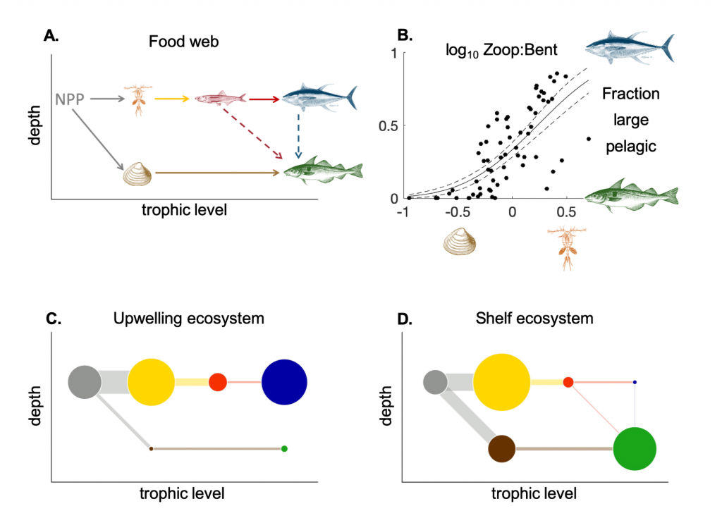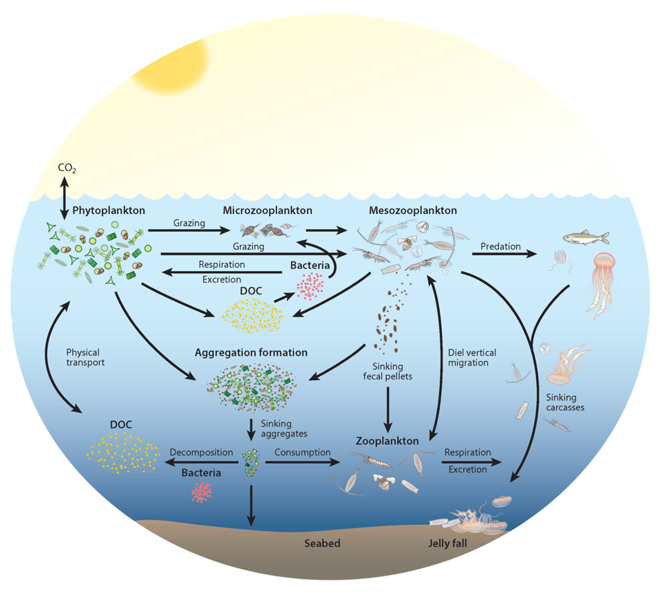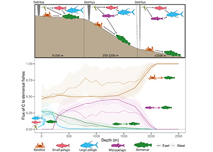
Ocean organisms transfer carbon via many natural processes from surface to seafloor. These include the passive sinking of carbon-rich particles and the active transport of carbon as animals swim downward. A recent study in GBC modeled how carbon stored in fish biomass moves from the sea surface to the seafloor in shelf–slope–abyssal systems through feeding interactions alone. This transport occurs as large fish eat smaller fish while occupying different vertical habitats in the water column. On average, this process delivers an amount equivalent to 5% of all carbon that reaches the seafloor—through sinking organic particles from phytoplankton and zooplankton. Yet, this can be as high as 20% in some shelf areas. On continental slopes, midwater fishes play a key role as a stepping-stone for carbon transfer (up to 50%) to the seafloor. Overall, the study reveals that the vertical movement of fish is an important pathway for delivering carbon to groundfish species, particularly on shelf areas where most commercially valuable fisheries operate.
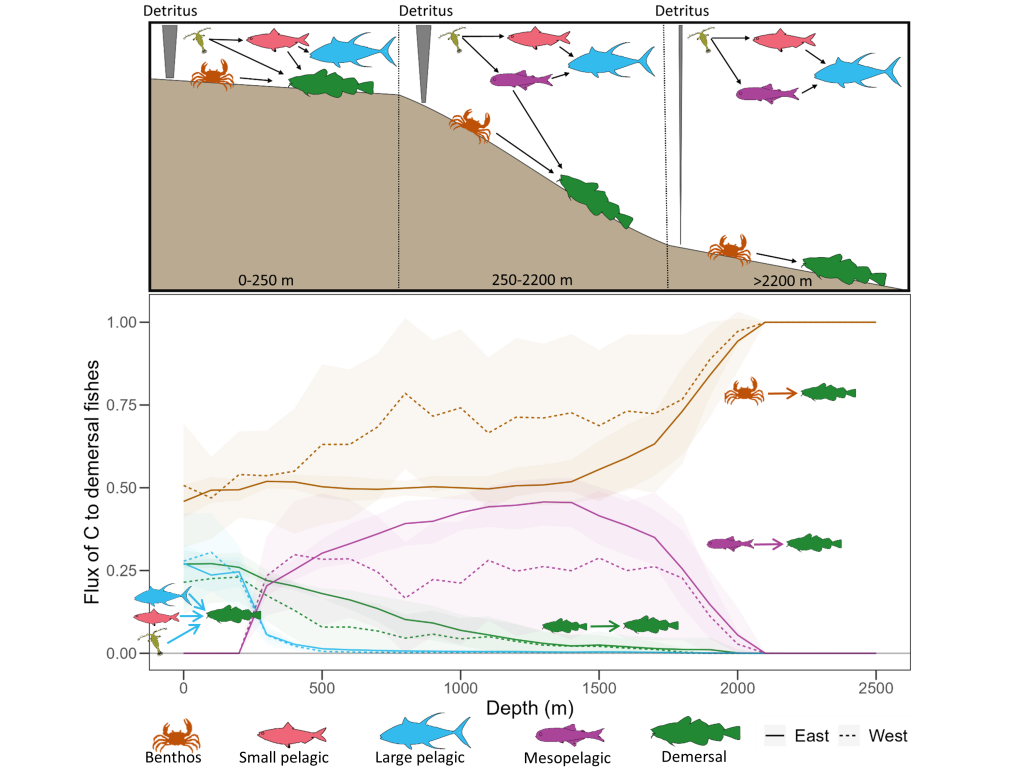
Caption: Schematic of a shelf-slope-abyssal system with hypothesized fluxes of carbon among major functional groups (top panel); and model-estimated fluxes of carbon from functional groups to demersal fishes (bottom panel). Solid and dotted lines are mean fluxes for Eastern and Western North Atlantic systems, respectively, and shaded areas are standard deviations. Values are proportional.
Authors
Daniel Ottmann (Technical University of Denmark (DTU-Aqua); Institute of Marine Sciences of Andalusia)
Ken H. Andersen (Technical University of Denmark (DTU-Aqua))
Yixin Zhao (Technical University of Denmark (DTU-Aqua))
Colleen M. Petrik (Scripps Institution of Oceanography)
Charles A. Stock (Scripps Institution of Oceanography)
Clive Trueman (University of Southampton)
P. Daniël van Denderen (Technical University of Denmark (DTU-Aqua))
Follow the authors:
bluesky: @danielottmann.bsky.social; @kenandersen.bsky.social
LinkedIn accounts: Ottman; Andersen; Truman
X: @daniel_ottmann; @69kno; @OceanLifeCenter; @van_denderen; @clivetrue;
Active Transport of Carbon to Demersal Fish Communities in Shelf-Slope-Abyssal Systems of the North Atlantic Ocean
Global Biogeochemical Cycles, Vol 40:2, e2025GB008861. https://doi.org/10.1029/2025GB008861