The global climate science community mourns the passing of Dr. Jorge Sarmiento in May 2026. In addition to co-authoring the first decadal U.S. Carbon Cycle Science Plan (Sarmiento and Wofsy, 1999) and leading the historic push to develop the U.S. Carbon Cycle Science Program and its carbon science coordination entities, OCB and NACP, Jorge stood as a pioneering “giant” in ocean biogeochemistry whose visionary leadership fundamentally shaped the trajectory of Earth system science. From his early steering of JGOFS to his profound contributions within OCB and his groundbreaking work heading the SOCCOM initiative, Jorge unraveled the critical complexities of the Southern Ocean and global marine ecosystems. Yet, beyond his extraordinary scientific accolades, including his shared recognition in the 2007 Nobel Peace Prize, his ultimate legacy lives on through his selfless mentorship, his infectious enthusiasm for new ideas, and the generations of brilliant scientists he inspired and guided. We owe an immeasurable debt of gratitude to Jorge for his career of profound discovery, collaborative spirit, and enduring dedication to understanding our planet. He will be deeply missed, but his scientific legacy remains a guiding light for all future carbon cycle research.
See also ‘Remembering Jorge Sarmiento, a ‘giant’ in climate studies’
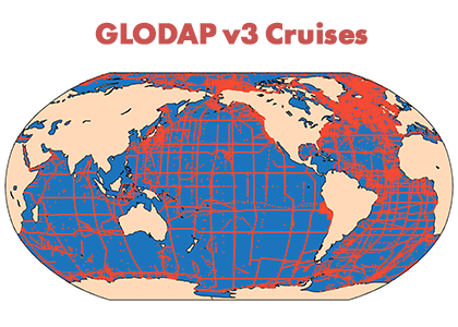
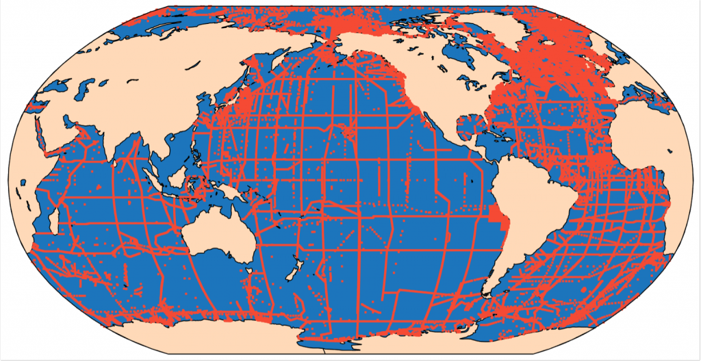
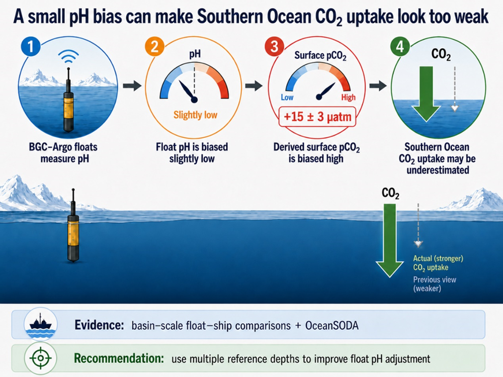
 On behalf of the GLODAP Reference Group and hundreds of seagoing oceanographers who have tirelessly collected data all over the ocean for several decades, it is our pleasure to announce the release of the new Global Ocean Data Analysis Project version 3, GLODAPv3!