air-sea interactions :: Ocean Carbon & Biogeochemistry

Studying marine ecosystems and biogeochemical cycles in the face of environmental change

Archive for air-sea interactions

Swirling Currents: How Ocean Mesoscale Affects Air-Sea CO2 Exchange

Posted by mmaheigan

· Friday, October 25th, 2024

Due to a sparsity of in‐situ observations and the computational burden of eddy‐resolving global simulations, there has been little analysis on how mesoscale processes (e.g., eddies, meanders—lateral scales of 10s to 100s km) influence air‐sea CO₂ fluxes from a global perspective. Recently, it became computationally feasible to implement global eddy‐resolving [O (10) km] ocean biogeochemical models. Many questions related to the influence of mesoscale motions on CO₂ fluxes remain open, including whether ocean eddies serve as hotspots for CO₂ sink or source in specific dynamic regions.

A recent study in Geophysical Research Letters investigated the contribution of ocean mesoscale variability to air-sea CO₂ fluxes by analyzing the CO₂ flux anomaly within the mesoscale band using a coarse-graining approach in a global eddy-resolving biogeochemical simulation. We found that in eddy-rich mid-latitude regions, ocean mesoscale variability can contribute to over 30% of the total CO₂ flux variability. The cumulative net CO₂ flux associated with mesoscale motions is on the order of 10⁵ tC per year. The global pattern of cumulative mesoscale-related CO₂ flux exhibits significant spatial heterogeneity, with the highest values in western boundary currents, the Antarctic Circumpolar Current, and the equatorial Pacific. The local distribution of cumulative mesoscale-related CO₂ flux displays zonal bands alternate between positive (a net source) and negative (a net sink) due to the meandering nature of ocean mesoscale currents, which is related to local relative vorticity and the background cross-stream pCO₂ gradient.

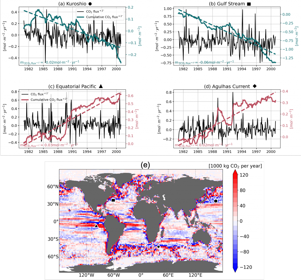
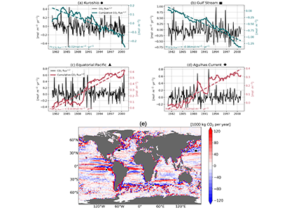
Figure caption. Mesoscale (<nominal 2 degree) contribution to air‐sea CO₂ flux (F^<2°_CO2)in the model. (a)–(d) Monthly time series of F^<2°_CO2 (black lines) and cumulative F^<2°_CO2 (green/red solid lines) in four locations marked in (e). Dashed lines are the least squares regression of cumulative flux for the period 1982–2000; slopes are indicated in the bottom left; (e) Blue colors imply a CO₂ sink, and red colors represent a source. The figure shows the global distribution of the regressed slopes of cumulative F^<2°_CO2. Units are converted from mol m^-2 per year to kg of CO₂ per year using the atomic mass of CO₂. This figure shows significant spatial heterogeneity of mesoscale-modulated CO₂ flux, showing contributions to both CO₂ sources and sinks across different regions of the ocean, with a magnitude on the order of 10⁵ tC per year.

Authors
Yiming Guo (Yale University; now at Woods Hole Oceanographic Institution)
Mary-Louise Timmermans (Yale University)

Towards using historical oxygen observations to reconstruct the air-sea flux of biological oxygen

Posted by mmaheigan

· Tuesday, December 13th, 2022

Dissolved oxygen (O₂) is a central observation in oceanography with a long history of relatively high precision measurements and increasing coverage over the 21^st century. O₂ is a powerful tracer of physical, chemical and biological processes (e.g., photosynthesis and respiration, wave-induced bubbles, mixing, and air-sea diffusion). A commonly used approach to partition the processes controlling the O₂ signal relies on concurrent measurements of argon (an inert gas), which has solubility properties similar to O₂. However, only a limited fraction of O₂ measurements have paired argon measurements.

Figure 1. (a) The newly developed empirical model to parameterize the physical oxygen saturation anomaly (ΔO_2[phy]) in order to separate the biological contribution from total oxygen, and (b-c) regional, inter-annual, and decadal variability of air-sea gas flux of biological oxygen (F[O2]bio as) reconstructed from the historical dissolved oxygen record.

A recent study published in the Journal of Global Biogeochemical Cycles presents semi-analytical algorithms to separate the biological and physical O₂ oxygen signals from O₂ observations. Among the approaches, a machine-learning algorithm using ship-based measurements and historical records of physical parameters from reanalysis products as predictors shows encouraging performance. The researchers leveraged this new algorithm to reconstruct regional, inter-annual, and decadal variability of the air-sea flux of biological oxygen (from historical O₂ records.

The long-term objective of this proof-of-concept effort is to estimate from historical oxygen records and a rapidly growing number of O₂ measurements on autonomous platforms. In regions where vertical and horizontal mixing is weak, the projected approximates net community production, providing an independent constraint on the strength of the biological carbon pump.

Authors:
Yibin Huang (Duke University)
Rachel Eveleth (Oberlin College)
David (Roo) Nicholson (Woods Hole Oceanographic Institution)
Nicolas Cassar (Duke University)

What drives decadal changes in the Chesapeake Bay carbonate system?

Posted by mmaheigan

· Tuesday, May 3rd, 2022

Understanding decadal changes in the coastal carbonate system (CO₂-system) is essential for predicting how the health of these waters is affected by anthropogenic drivers, such as changing atmospheric conditions and terrestrial inputs. However, studies that quantify the relative impacts of these drivers are lacking.

A recent study in Journal of Geophysical Research: Oceans identified the primary drivers of acidification in the Chesapeake Bay over the past three decades. The authors used a three-dimensional hydrodynamic-biogeochemistry model to quantify the relative impacts on the Bay CO₂-system from increases in atmospheric CO₂, temperature, oceanic dissolved inorganic carbon (DIC) concentrations, terrestrial loadings of total alkalinity (TA) and DIC, as well as decreases in terrestrial nutrient inputs. Decadal changes in the surface CO₂-system in the Chesapeake Bay exhibit large spatial and seasonal variability due to the combination of influences from the land, ocean and atmosphere. In the upper Bay, increased riverine TA and DIC from the Susquehanna River have increased surface pH, with other drivers only contributing to decadal changes that are one to two orders of magnitude smaller. In the mid- and lower Bay, higher atmospheric CO₂ concentrations and reduced nutrient loading are the two most critical drivers and have nearly equally reduced surface pH in the summer. These decadal changes in surface pH show significant seasonal variability with the greatest magnitude generally aligning with the spring and summer shellfish production season (Figure 1).

Figure 1: Overall changes in modeled surface pH (ΔpH_all) due to all global and terrestrial drivers combined over the past 30 years (i.e., 2015–2019 relative to 1985–1989). ΔpH_all includes changes in surface pH due to increased atmospheric CO2, increased atmospheric thermal forcing, increased oceanic dissolved inorganic carbon concentrations, decreased riverine nitrate concentrations, decreased riverine organic nitrogen concentrations, and increased riverine total alkalinity and dissolved inorganic carbon concentrations.

These results indicate that a number of global and terrestrial drivers play crucial roles in coastal acidification. The combined effects of the examined drivers suggest that calcifying organisms in coastal surface waters are likely facing faster decreasing rates of pH than those in open ocean ecosystems. Decreases in surface pH associated with nutrient reductions highlight that the Chesapeake Bay ecosystem is returning to a more natural condition, e.g., a condition when anthropogenic nutrient input from the watershed was lower. However, increased atmospheric CO₂ is simultaneously accelerating the rate of change in pH, exerting increased stress on estuarine calcifying organisms. For ecosystems such as the Chesapeake Bay where nutrient loading is already being managed, controlling the emissions of anthropogenic CO₂ globally becomes increasingly important to decelerate the rate of acidification and to relieve the stress on estuarine calcifying organisms. Future observational and modeling studies are needed to further investigate how the decadal trends in the Chesapeake Bay CO₂-system may vary with depth. These efforts will improve our current understanding of long-term change in coastal carbonate systems and their impacts on the shellfish industry.

Authors:
Fei Da (Virginia Institute of Marine Science, William & Mary, USA)
Marjorie A. M. Friedrichs (Virginia Institute of Marine Science, William & Mary, USA)
Pierre St-Laurent (Virginia Institute of Marine Science, William & Mary, USA)
Elizabeth H. Shadwick (CSIRO Oceans and Atmosphere, Australia)
Raymond G. Najjar (The Pennsylvania State University, USA)
Kyle E. Hinson (Virginia Institute of Marine Science, William & Mary, USA)

Contrasting N2O fluxes of source vs. sink in western Arctic Ocean during summer 2017

Posted by mmaheigan

· Wednesday, October 20th, 2021

During the western Arctic summer season both physical and biogeochemical features differ with latitude between the Bering Strait and Chukchi Borderland. The southern region (Bering Strait to the Chukchi Shelf) is relatively warm, saline, and eutrophic, due to the intrusion of Pacific waters that bring heat and nutrients in to the western Arctic Ocean (WAO). Because of the Pacific influence, the WAO is one of the most productive stretches of ocean in the world. In contrast, the northern region (Chukchi Borderland to the Canada Basin) is primarily influenced by freshwater originating from sea ice melt and rivers, and is relatively cold, fresh, and oligotrophic. A frontal zone exists between the southern region and northern region (~73°N) due to the distinct physicochemical contrast between mixing Pacific waters and freshwater. These regions support distinct bacterial communities also, making the environmental variations drivers extremely relevant to nitrous oxide (N₂O) dynamics.

A recent study published in Scientific Reports examined the role of the WAO as a source and a sink of atmospheric N₂O. There are obvious differences in N₂O fluxes between southern Chukchi Sea (SC) and northern Chukchi Sea (NC). In the SC (Pacific water characteristics dominate) N₂O emissions act as a net source to the atmosphere (Figure 1a). In the NC (freshwater dominant) absorption of atmospheric N₂O into the water column suggests that this region acts as a net sink (Figure 1a). The positive fluxes of SC occurred with relatively high sea surface temperature (SST), sea surface salinity (SSS), and biogeochemically-derived N₂O production, whereas the negative fluxes of NC were associated with relatively low SST, SSS, and little N₂O production. These linear relationships between N₂O fluxes and environmental variables suggest that summer WAO N₂O fluxes are remarkably sensitive to environmental changes.

Figure 1. (a) Map of the sampling stations using the Ice Breaking R/V Araon during August 2017. The sampling locations were coloured with N2O fluxes (blue to red gradient, see color bar; sink, air → sea (−), and source, sea → air (+). The southern Chukchi Sea (SC) extends from Bering Strait to Chukchi Shelf and the northern Chukchi Sea (NC) extends from Chukchi Borderland and Canada Basin. The frontal zone arises between SC and NC (black dotted line). (b) Illustration showing future changes in the distribution of the WAO N2O flux constrained by the positive feedback scenario of increasing inflow of Pacific waters and rapidly declining sea-ice extent under accelerating Arctic warming.

This study suggests a potential scenario for future WAO changes in terms of accelerating Arctic change. Increasing inflow of the Pacific waters and rapidly declining sea-ice extent are critical. The increasing inflow of warm nutrient-enriched Pacific waters will likely extend the SC N₂O source region northward, increasing productivity, and thereby intensifying nitrification. All of which would lead to a strengthening of the WAO’s role as an N₂O source. A rapid loss of the sea ice extent could ultimately lead to a sea-ice-free NC, and again, a northward shift, which would result in a diminished role of the NC as an N₂O sink (Figure 1b). While improving our understanding of WAO N₂O dynamics, this study suggests both a direction for future work and a clear need for a longer-term study to answer questions about both seasonal variations in these dynamics and possible interannual to climatological trends.

Authors:
Jang-Mu Heo (Department of Marine Science, Incheon National University)
Sang-Min Eom (Department of Marine Science, Incheon National University)
Alison M. Macdonald (Woods Hole Oceanographic Institution)
Hyo-Ryeon Kim (Department of Marine Science, Incheon National University)
Joo-Eun Yoon (Department of Marine Science, Incheon National University)
Il-Nam Kim (Department of Marine Science, Incheon National University)

Acidity across the interface from the ocean surface to sea spray aerosol

Posted by mmaheigan

· Wednesday, March 31st, 2021

The pH of aerosols controls their impact on climate and human health. Sea spray aerosols are one of the largest sources of aerosols globally by mass, yet it has been challenging to measure the pH of fresh sea spray aerosols in the past. A recent study published in PNAS measured sea spray aerosols under controlled conditions, during a sampling intensive called SeaSCAPE, and optimized a pH paper-based technique to measure the aerosol acidity. The authors found that fresh sea spray aerosols can be rapidly acidified by 4 to 6 orders of magnitude relative to the ocean. This acidification is caused by interaction with surrounding acidic gases, changes in relative humidity, and enhanced dissociation of organic acids within the aerosols. This is a critical finding since the pH of aerosols controls key atmospheric chemical reactions including sulfur dioxide oxidation to form particulate sulfate. The results are also important in light of the fact that enzyme activity has been observed in sea spray aerosols, and enzyme activity is pH dependent.

Figure 1. Acidity of nascent sea spray aerosols (SSA) compared to bulk ocean water measured during the 2019 SeaSCAPE sampling intensive. Background artwork by Nigella Hillgarth.

Authors
Kyle Angle (University of California, San Diego)
Daniel Crocker (University of California, San Diego)
Rebecca Simpson (University of California, San Diego)
Kathryn Mayer (University of California, San Diego)
Lauren Garofalo (Colorado State University, Fort Collins)
Alexia Moore (University of California, San Diego)
Stephanie Mora Garcia (University of California, San Diego)
Victor Or (University of California, San Diego)
Sudarshan Srinivasan (University of California, San Diego)
Mahum Farhan (University of California, San Diego)
Jonathan Sauer (University of California, San Diego)
Christopher Lee (University of California, San Diego)
Matson Pothier (Colorado State University, Fort Collins)
Delphine Farmer (Colorado State University, Fort Collins)
Todd Martz (University of California, San Diego)
Timothy Bertram (University of Wisconsin, Madison)
Christopher Cappa (University of California, Davis)
Kimberly Prather (University of California, San Diego)
Vicki Grassian (University of California, San Diego)

Joint post with Surface Ocean – Lower Atmosphere Study (SOLAS)

Air-sea gas disequilibrium drove deoxygenation of the deep ice-age ocean

Posted by mmaheigan

· Thursday, March 18th, 2021

During the Last Glacial Maximum (~20,000 years ago, LGM) sediment data show that the deep ocean had lower dissolved oxygen (O₂) concentrations than the preindustrial ocean, despite cooler temperatures of this period increasing O₂ solubility in sea water.

Figure 1. a) Whole ocean inventory of the O₂ components in the preindustrial control (PIC): total O₂ (O₂); the preformed components equilibrium O₂ (O₂ equilibrium), physical disequilibrium O₂ (O₂ diseq phys) and biologically-mediated disequilibrium (O₂ diseq bio); and O₂ respired from soft-tissue (O₂ soft). b) The difference in whole ocean inventory of O₂ components between the LGM and PIC simulations.

In a study published in Nature Geoscience, the authors provide one of the first explanations for glacial deoxygenation. The authors combined a data-constrained model of the preindustrial (PIC) and LGM ocean with a novel decomposition of O₂ to assess the processes affecting the oceanic distribution of oxygen. The decomposition allowed for the preformed disequilibrium O₂—the amount of oxygen that deviates from its solubility equilibrium value when at the surface—to be tracked, along with other contributions such as the O₂ consumed by bacterial respiration of organic matter. In the preindustrial ocean, a third of the subsurface oxygen deficit was a result of disequilibrium rather than oxygen consumed by bacteria. This contradicts previous assumptions (Figure 1a). Nearly 80% of the disequilibrium resulted from upwelling waters, depleted in O₂ due to respiration, not fully equilibrating before re-subduction into the ocean interior. This effect was even greater during the LGM (Figure 1b). The authors attributed this largely to the widespread presence of sea ice—which acts as a cap on the surface preventing the water from gaining oxygen from the atmosphere—in the ocean around Antarctica, with a smaller contribution from iron fertilization.

This study provides one of the first mechanistic explanations for LGM deep ocean deoxygenation. As the ocean is currently losing oxygen due to warming, the effect of other processes, including sea ice changes, could prove important for understanding long-term ocean oxygenation changes.

Authors
Ellen Cliff (University of Oxford)
Samar Khatiwala (University of Oxford)
Andreas Schmittner (Oregon State University)

Joint highlight with GEOTRACES International Project Office

A new Regional Earth System Model of the Mediterranean Sea biogeochemical dynamics

Posted by mmaheigan

· Thursday, November 19th, 2020

The Mediterranean Sea is a semi-enclosed mid-latitude oligotrophic basin with a lower net primary production than the global ocean. A west-east productivity trophic gradient results from the superposition of biogeochemical and physical processes, including the biological pump and associated carbon and nutrient (nitrogen, phosphorus) fluxes, the spatial asymmetric distribution of nutrient sources (rivers, atmospheric deposition, coastal upwelling, etc.), the estuarine inverse circulation associated with the inflow of Atlantic water through the Gibraltar Strait. The complex and highly variable interface between land and sea throughout this basin add a further layer of complexity in the Mediterranean oceanic and atmospheric circulation and on the associated biogeochemistry dynamics, emphasizing the need for high-resolution truly integrated Regional Earth System Models to track and understand fine-scale processes and ecosystem dynamics.

In a recent paper published in the Journal of Advances in Modeling Earth System, the authors introduced a new version of the Regional Earth System model RegCM-ES and evaluated its performance in the Mediterranean region. RegCM-ES fully integrates the regional climate model RegCM4, the land surface scheme CLM4.5 (Community Land Model), the river routing model HD (Hydrological Discharge Model), the ocean model MITgcm (MIT General Circulation model) and the Biogeochemical Flux Model BFM.

A comparison with available observations has shown that RegCM-ES was able to capture the mean climate of the region and to reproduce horizontal and vertical patterns of chlorophyll-a and PO₄(the limiting nutrient in the basin) (Figure 1). The same comparison revealed a systematic underestimation of simulated dissolved oxygen (which will be fixed by the use of a new parametrization of oxygen solubility), and an overestimation of NO₃, possibly due to uncertainties in initial and boundary conditions (mostly traced to river and Dardanelles nutrient discharges) and an overly vigorous vertical mixing simulated by the ocean model in some parts of the Basin.

Figure.1 Distributions of chlorophyll-a mg/m³ (top) and PO₄ mmol/m³ (bottom) in the Mediterranean Sea as simulated by RegCM-ES.

Overall, this analysis has demonstrated that RegCM-ES has the capabilities required to become a powerful tool for studying regional dynamics and impacts of climate change on the Mediterranean Sea and other ocean basins around the world.

Authors:
Marco Reale (Abdus Salam International Centre for theoretical physics-ICTP, National Institute of Oceanography and Experimental Geophysics-OGS)
Filippo Giorgi (Abdus Salam International Centre for theoretical physics-ICTP)
Cosimo Solidoro (National Institute of Oceanography and Experimental Geophysics-OGS)
Valeria Di Biagio (National Institute of Oceanography and Experimental Geophysics-OGS)
Fabio Di Sante (Abdus Salam International Centre for theoretical physics-ICTP)
Laura Mariotti (National Institute of Oceanography and Experimental Geophysics-OGS)
Riccardo Farneti (Abdus Salam International Centre for theoretical physics-ICTP)
Gianmaria Sannino (Italian National Agency for New Technologies, Energy and Sustainable Economic Development-ENEA)

Will global change “stress out” ocean DOC cycling?

Posted by mmaheigan

· Tuesday, September 29th, 2020

The dissolved organic carbon (DOC) pool is vital for the functioning of marine ecosystems. DOC fuels marine food webs and is a cornerstone of the earth’s carbon cycle. As one of the largest pools of organic matter on the planet, disruptions to marine DOC cycling driven by climate and environmental global changes can impact air-sea CO2 exchange, with the added potential for feedbacks on Earth’s climate system.

Figure 1. Simplified view of major dissolved organic carbon (DOC) sources (black text) and sinks (yellow text) in the ocean.

Since DOC cycling involves multiple processes acting concurrently over a range of time and space scales, it is especially challenging to characterize and quantify the influence of global change. In a recent review paper published in Frontiers in Marine Science, the authors synthesize impacts of global change-related stressors on DOC cycling such as ocean warming, stratification, acidification, deoxygenation, glacial and sea ice melting, inflow from rivers, ocean circulation and upwelling, and atmospheric deposition. While ocean warming and acidification are projected to stimulate DOC production and degradation, in most regions, the outcomes for other key climate stressors are less clear, with much more regional variation. This synthesis helps advance our understanding of how global change will affect the DOC pool in the future ocean, but also highlights important research gaps that need to be explored. These gaps include for example a need for studies that allow to understand the adaptation of degradation/production pathways to global change stressors, and their cumulative impacts (e.g. temperature with acidification).

Authors:
C. Lønborg (Aarhus University)
C. Carreira (CESAM, Universidade de Aveiro)
Tim Jickells (University of East Anglia)
X.A. Álvarez-Salgado (CSIC, Instituto de Investigacións Mariñas)

Unexpected patterns of carbon export in the Southern Ocean

Posted by mmaheigan

· Tuesday, July 7th, 2020

The Southern Ocean is a major player in driving global distributions of heat, carbon dioxide, and nutrients, making it key to ocean chemistry and the earth’s climate system. In the ocean, biological production and export of organic carbon are commonly linked to places with high nutrient availability. A recent paper, published in Global Biogeochemical Cycles, highlighting new observations from robotic profiling floats demonstrates that areas of high carbon export in the Southern Ocean are actually associated with very low concentrations of iron, an important micronutrient for supporting phytoplankton growth. This suggests a decoupling between the production and export of organic carbon in this region.

Figure caption: (A) Meridional pattern of Annual Net Community Production (ANCP) (equivalent to carbon export) (± standard deviation) in the Southern Ocean (blue line with circles and shaded area), carbon export estimates from previous satellite-based analyses (blue dashed line), and silicate to nitrate (Si:NO₃) ratio of the surface water (black continuous line). Grey dotted line shows a Si:NO₃ = 1 mol mol⁻¹, characteristic of nutrient-replete diatoms. (B) Meridional pattern of Southern Ocean nutrient concentrations, including dissolved iron (Fe) concentration (black line), nitrate (red line), and silicate (blue line). (C) Mean 2014–2015 annual zonally averaged air-sea flux of CO₂ computed using neural network interpolation method. STF = Subtropical Front, PF = Antarctic Polar Front, SIF = Seasonal Ice Front.

Using observations of nutrient and oxygen drawdown from a regional network of profiling Biogeochemical-Argo floats deployed as part of the Southern Ocean Carbon and Climate Observations and Modeling project (SOCCOM), the authors calculated estimates of Southern Ocean carbon export. A meridional pattern in biological carbon export emerged, showing peak export near the Antarctic Polar Front (PF) associated with minima in surface iron concentrations and dissolved silicate to nitrate ratios. Previous studies have shown that under iron-limiting conditions, diatoms increase their uptake ratio of silicate with respect to other nutrients (e.g., nitrogen), resulting in silicification. Here, the authors hypothesize that iron limitation promotes silicification in Southern Ocean diatoms, as evidenced by the low silicate to nitrate ratio of surface waters around the Antarctic Polar Front. High diatom silicification increases ballasting of particulate organic carbon and hence overall carbon export in this region. The resulting meridional pattern of organic carbon export is similar to that of the air-sea flux of carbon dioxide in the Southern Ocean, underscoring the importance of the biological carbon pump in controlling the spatial pattern of oceanic carbon uptake in this region.

Authors:
Lionel A. Arteaga (Princeton University)
Markus Pahlow (Helmholtz Centre for Ocean Research Kiel, GEOMAR)
Seth M. Bushinsky (University of Hawaii)
Jorge L. Sarmiento (Princeton University)

Arctic rivers as carbon highways

Posted by mmaheigan

· Tuesday, June 16th, 2020

Rapid environmental changes in the Arctic will potentially alter the atmospheric emissions of heat-trapping greenhouse gases such as methane (CH₄) and carbon dioxide (CO₂). A recent study on the Canadian Arctic published in Geophysical Research Letters reveals that spring meltwater delivery drives episodic outgassing events along the lake-river-bay continuum. This spring runoff period is not well-represented in prior studies, which, due to ease of sampling access, have focused more on summertime low-ice conditions. Study authors established a community-based monitoring program in Cambridge Bay and an adjacent inflowing river system in Nunavut, Canada from 2017-2018. These time-series data revealed that at the onset of the melt season river water contains methane concentrations up to 2000 times higher than observed in the bay from late summer through early spring (Figure 1 panel a). In addition, the authors deployed a novel robotic chemical sensing kayak (the ChemYak) in the Bay for five days in 2018 to densely sample water CH₄and CO₂levels in space and time during the spring thaw (Figure 1 panel b). The ChemYak observations revealed that river water containing elevated levels of both of these greenhouse gases flowed into the bay and outgassed to the atmosphere over a period of 5 days! The authors estimate that river inflow during the short melt season drives >95% of all annual methane emissions from the bay. These results demonstrate the need for seasonally-resolved sampling to accurately quantify greenhouse gas emissions from polar systems.

Figure 1: Panel a) Measurements of methane concentration in Cambridge Bay and an adjacent river showed strong seasonality; elevated concentrations were associated with river inflow at the start of the freshet. Panel b) Observations with the ChemYak robotic surface vehicle in Cambridge Bay revealed that excess methane was rapidly ventilated to the atmosphere following ice melt in the bay.

Authors
Cara Manning (University of British Columbia)
Victoria Preston (Woods Hole Oceanographic Institution and Massachusetts Institute of Technology)
Samantha Jones (University of Calgary)
Anna Michel (Woods Hole Oceanographic Institution)
David Nicholson (Woods Hole Oceanographic Institution)
Patrick Duke (University of Calgary and University of Victoria)
Mohamed Ahmed (University of Calgary)
Kevin Manganini (Woods Hole Oceanographic Institution)
Brent Else (University of Calgary)
Philippe Tortell (University of British Columbia)

Funding for the Ocean Carbon & Biogeochemistry Project Office is provided by the National Science Foundation (NSF) and the National Aeronautics and Space Administration (NASA). The OCB Project Office is housed at the Woods Hole Oceanographic Institution.

Archive for air-sea interactions

Filter by Keyword