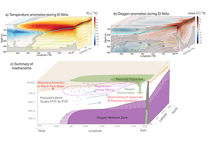
What drives the year-to-year variability of dissolved oxygen (O2) in the tropical Pacific? A recent study explored this question using a global high-resolution model with active ocean biogeochemistry along with a machine learning based estimate of dissolved oxygen from Argo floats. El Niño and La Niña events play a major role in regulating the O2 content and distribution in the tropical Pacific. El Niño events result in excess O2 in the eastern tropical Pacific and reduced O2 in the west. La Niña yields opposite patterns. In contrast to previous speculations that lower model resolution leads to an underestimate of observed O2 variability in this region, we find little difference in the amplitude of the O2 content change between models of different resolution (~1º vs 0.1º) and the observations-based machine learning estimate. ENSO-driven variability of O2 in the eastern tropical Pacific is driven by large opposing physical and biological contributions: reduced upwelling of low-O2 waters and weaker O2 consumption at depth due to suppressed biological productivity during El Niño dominate over the reduction in O2 ventilation by vertical turbulent mixing and the Equatorial Undercurrent, and the opposite occurs during La Niña. This subtle balance between competing processes suggests that future changes in O2 in the tropical Pacific are likely to be sensitive to local changes in equatorial Pacific circulation and productivity, in addition to changes in large scale O2 supply from the mid and high latitude basins as the ocean warms and stratifies. These O2 changes have important implications for understanding and predicting marine ecosystem health and fisheries productivity throughout the tropical Pacific.
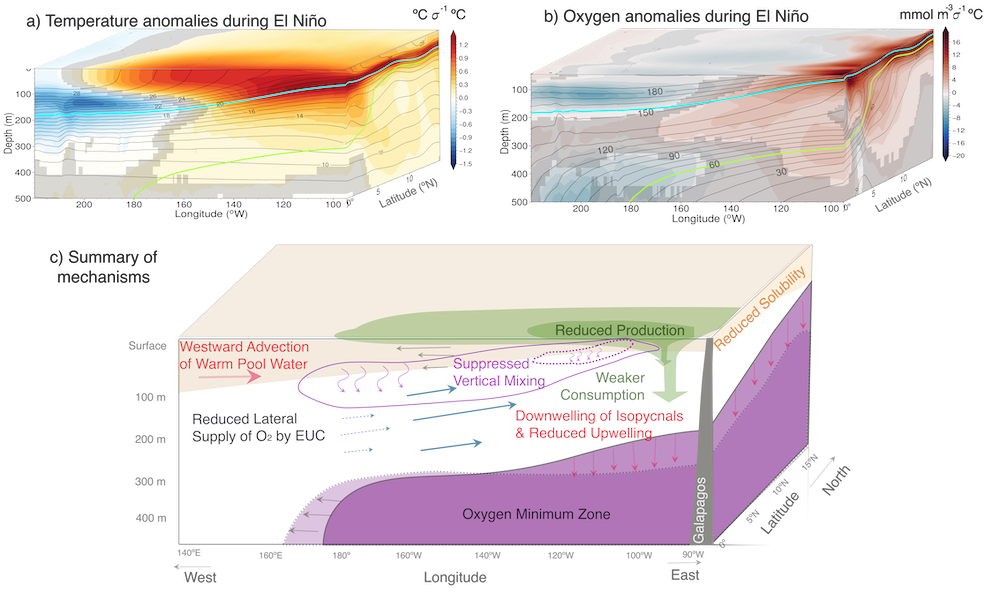
Figure: ENSO impacts on temperature and O2 shown as regression of Nino 3.4 index on a) temperature anomalies, and b) O2 anomalies in a high resolution simulation of CESM. Panel c) illustrates the main mechanisms governing the O2 response to El Niño events.
Authors
Yassir A. Eddebbar (Scripps Institution of Oceanography)
M L. Hoffman (Scripps Institution of Oceanography)
Jonathan D. Sharp (UW/NOAA)
Daniel B. Whitt (NASA Ames)
Aneesh C. Subramanian (CU Boulder)
Sam Stevenson (UC Santa Barbara)
@NCAR_CGD @CUBoulderATOC @Scripps_Ocean @aneeshcs @CLIVAR @USCLIVAR
Citation: Eddebbar, Y. A., Hoffman, E. L., Sharp, J. D., Whitt, D. B., Subramanian, A. C., & Stevenson, S. (2026). ENSO-Driven Variability of Oxygen Content and Distribution in the Tropical Pacific. Journal of Climate, 39(5), 1333-1353. https://doi.org/10.1175/JCLI-D-25-0476.1