How much carbon do ocean eddies actually pump into the ocean interior? A decade ago, a landmark study (Omand et al, 2015) showed that turbulent eddies at ocean fronts can grab carbon-rich surface water and plunge it hundreds of meters down in a matter of days—back-of-the-envelope extrapolations suggest this “eddy subduction pump” could export as much as 2 Pg of carbon per year (Boyd et al, 2019), roughly a fifth of the entire biological carbon pump. But because these events are small, short-lived, and scattered across every ocean basin, constraining the pump’s true size at the global scale has remained elusive. The authors of a recent study built an algorithm that detects individual subduction events from coincident anomalies in salinity, oxygen, and particulate organic carbon, and applied this algorithm to 126,591 profiles from 941 BGC-Argo floats, identifying 1,333 carbon subduction events concentrated in springtime hotspots in the Southern Ocean and the subpolar North Atlantic. The resulting global export below 200 m is about 0.05 [<0.01–0.28] Pg C yr⁻¹, orders of magnitude smaller than the earlier upper bound, and less than 5% of the total biological pump. The result is in close agreement with an independent global estimate derived from a four-dimensional POC budget (Bellacicco et al., 2025), giving us added confidence that the pump’s true magnitude is modest. This is, somewhat counterintuitively, reassuring news for global carbon budgets. Current Earth System Models cannot resolve the kilometer-scale dynamics behind eddy subduction, but our results suggest they are not missing a first-order term in the ocean carbon cycle.
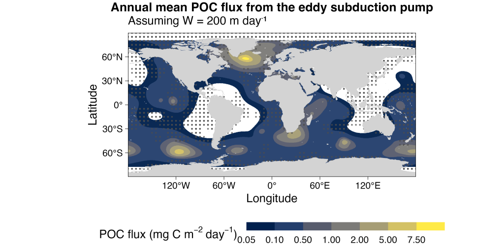
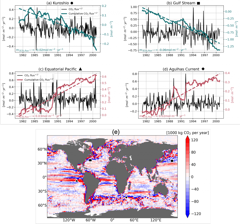
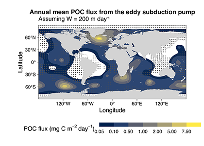
Figure caption : Spatial distribution of total annual mean POC flux below 200 m from the eddy subduction pump, assuming a constant vertical velocity W = 200 m day⁻¹. Strongest export occurs in the Southern Ocean and subpolar North Atlantic. White stippling marks 5° grid cells without Argo profiles (insufficient coverage).
Authors
Maxime Keutgen De Greef
Laure Resplandy
Mathieu A. Poupon
(all Princeton Univ)