Polar regions are changing: warming, losing sea ice, and experiencing shifts in the phenology of seasonal events. Global models predict that phytoplankton blooms will start earlier in these warming polar environments. What we don’t know is will this be true for all high-latitude regions? Is the timing of phytoplankton growing season moving earlier in the West Antarctic Peninsula as this region experiences climate change?
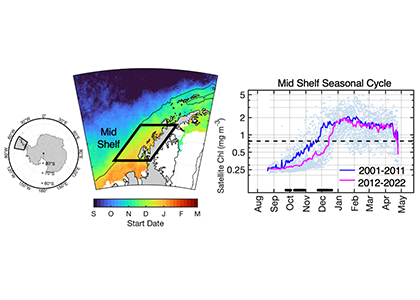
The authors of a recent paper published in Marine Ecology Progress Series used 25 years of satellite ocean color data to track shifts in bloom phenology—the timing of recurring seasonal events. Contrary to predictions, the results show that the spring bloom start date is shifting later over time. Figure 1 shows that in the waters experiencing seasonal sea ice, from 1997 to 2022, the start and peak date of the phytoplankton growing season are shifting later. However, there is no overall decline in total annual chlorophyll-a, because in the fall (February-April) chlorophyll-a concentrations are increasing over time.
The most likely driver of earlier spring bloom start dates is increased wind mixing. Spring (October-December) wind speed has been increasing over time concurrent with delayed bloom start dates. In an ecosystem with less sea ice than previous decades, more open water exposed to increased wind speed may mix phytoplankton more deeply in spring, delaying the bloom until the onset of summer stratification.
Even though global climate models predict bloom timing will shift earlier with climate change, this may not be the case in specific polar regions like the West Antarctic Peninsula. Later bloom timing could impact surface ocean carbon uptake, phytoplankton community composition, and ecosystem health. If the timing and composition of blooms is changing, that shifts will affect the food quantity and quality available to krill and higher trophic level organisms.
Author
Jessie Turner (University of Connecticut) @jessiesturner
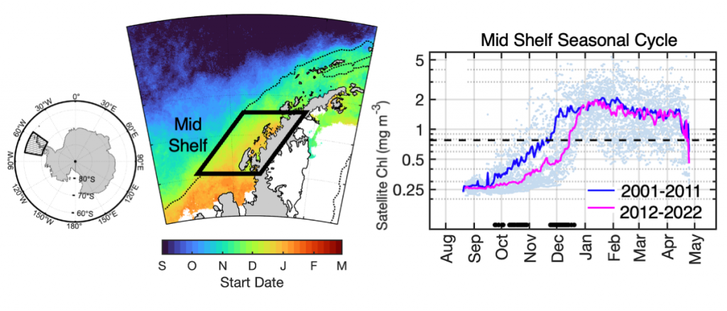
Figure 1: In recent years the timing of the annual phytoplankton bloom in the Mid Shelf region of the West Antarctic Peninsula has shifted: satellite-derived chlorophyll-a concentration in recent years (pink line) shows a significant delayed bloom start date compared to past years (blue line).