oxygen :: Ocean Carbon & Biogeochemistry

Studying marine ecosystems and biogeochemical cycles in the face of environmental change

Archive for oxygen

Quantifying uncertainties in future projections of Chesapeake Bay Hypoxia

Posted by mmaheigan

· Wednesday, December 4th, 2024

Climate change is expected to especially impact coastal zones, worsening deoxygenation in the Chesapeake Bay by reducing oxygen solubility and increasing remineralization rates of organic matter. However, simulated responses of this often fail to account for uncertainties embedded within the application of future climate scenarios.

Recent research published in Biogeosciences and in Scientific Reports sought to tackle multiple sources of uncertainty in future impacts to dissolved oxygen levels by simulating multiple climate scenarios within the Chesapeake Bay region using a coupled hydrodynamic-biogeochemical model. In Hinson et al. (2023), researchers showed that a multitude of climate scenarios projected a slight increase in hypoxia levels due solely to watershed impacts, although the choice of global earth system model, downscaling methodology, and watershed model equally contributed to the relative uncertainty in future hypoxia estimates. In Hinson et al. (2024), researchers also found that the application of climate change scenario forcings itself can have an outsized impact on Chesapeake Bay hypoxia projections. Despite using the same inputs for a set of three experiments (continuous, time slice, and delta), the more commonly applied delta method projected an increase in levels of hypoxia nearly double that of the other experiments. The findings demonstrate the importance of ecosystem model memory, and fundamental limitations of the delta approach in capturing long-term changes to both the watershed and estuary. Together these multiple sources of uncertainty interact in unanticipated ways to alter estimates of future discharge and nutrient loadings to the coastal environment.

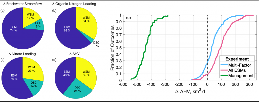
Figure 1: Chesapeake Bay hypoxia is sensitive to multiple sources of uncertainty related to the type of climate projection applied and the effect of management actions. Percent contribution to uncertainty from Earth System Model (ESM), downscaling methodology (DSC), and watershed model (WSM) for estimates of (a) freshwater streamflow, (b) organic nitrogen loading, (c) nitrate loading, and (d) change in annual hypoxic volume (ΔAHV). (e) Summary of all experiment results for ΔAHV, expressed as a cumulative distribution function. The Multi-Factor experiment (blue line) used a combination of multiple ESMs, DSCs, and WSMs, the All ESMs experiment (pink line) simulated 20 ESMs while holding the DSC and WSM constant, and the Management experiment (green line) only simulated 5 ESMs with a single DSC and WSM but incorporated reductions in nutrient inputs to the watershed. The vertical dashed black line marks no change in AHV.

Understanding the relative sources of uncertainty and impacts of environmental management actions can improve our confidence in mitigating negative climate impacts on coastal ecosystems. Better quantifying contributions of model uncertainty, that is often unaccounted for in projections, can constrain the range of outcomes and improve confidence in future simulations for environmental managers.

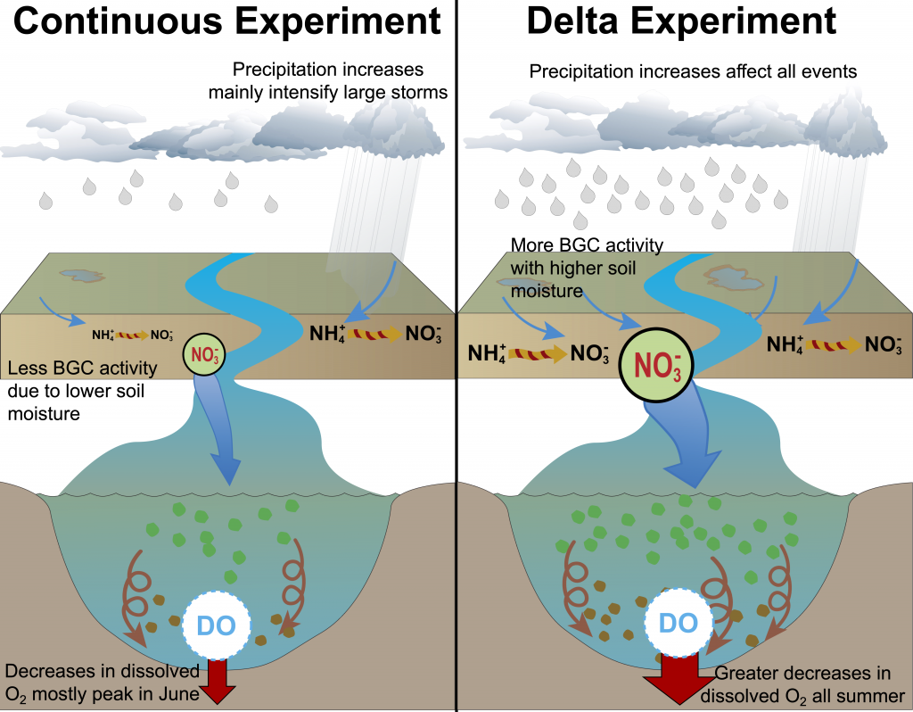
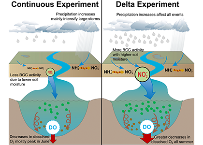
Figure 2: A schematic of differences between the Continuous and Delta experiments. In the Delta experiment a combination of altered distributions in future precipitation and changes to long-term soil nitrogen stores eventually result in increased levels of hypoxia (right panel).

Authors
Kyle E. Hinson (Virginia Institute of Marine Science, William & Mary)
Marjorie A. M. Friedrichs (Virginia Institute of Marine Science, William & Mary)
Raymond G. Najjar (The Pennsylvania State University)
Maria Herrmann (The Pennsylvania State University)
Zihao Bian (Auburn University)
Gopal Bhatt (The Pennsylvania State University, USEPA Chesapeake Bay Program Office)
Pierre St-Laurent (Virginia Institute of Marine Science, William & Mary)
Hanqin Tian (Boston College)
Gary Shenk (USGS Virginia/West Virginia Water Science Center)

Turbulent Mixing: A Dominant Source of Oxygen in the Upper Equatorial Pacific

Posted by mmaheigan

· Tuesday, March 12th, 2024

What balances oxygen removal in the equatorial Pacific? For a long time, oxygen in the eastern and central tropical Pacific was assumed to be mainly supplied by the large-scale advection of remotely ventilated waters via the equatorial current system and meridional circulation. A recent study used an eddy-resolving simulation of a global ocean model to show that turbulent mixing and its regulation by mesoscale eddies play a critical role in balancing oxygen removal (by consumption and upwelling) in the upper thermocline. Deeper in the water column, mean advection by the zonal currents and meridional circulation dominates. This mixing is tightly regulated by tropical instability waves, which intensify the shear between the equatorial currents and enhance the downward turbulent mixing flux of oxygen into the thermocline. Mesoscale phenomena thus play an indirect yet critical role as a local pathway of ventilation in this region. Testing these model-based hypotheses in the real ocean through dedicated field studies and long-term observations is needed to advance our understanding of the observed expansion of the oxygen deficient zones (ODZs) and model their future trajectory in a warmer and more stratified ocean.

Figure: The main processes that set the mean structure of oxygen in the equatorial Pacific are assessed in an eddy resolving simulation of the Community Earth System Model (CESM). Panel a shows the climatological oxygen distribution on the 26.25 isopycnal in CESM. Panels b-e show the contribution of advection by mean circulation and eddies, vertical mixing, and production and consumption. These processes are illustrated in panel f). Figure adapted from Eddebbar et al (2024).

Authors
Yassir A. Eddebbar (Scripps Institution of Oceanography)
Daniel B. Whitt (NASA Ames)
Ariane Verdy, (Scripps Institution of Oceanography)
Matthew R. Mazloff (Scripps Institution of Oceanography)
Aneesh C. Subramanian (CU Boulder)
Matthew C. Long, (National Center for Atmospheric Research)

Identifying the water mass composition of a sample has never been so easy!

Posted by mmaheigan

· Thursday, August 31st, 2023

When we collect seawater in any point of the ocean, we are collecting a mix of water masses from different origin that traveled until there keeping their salinity and temperature properties. The Atlantic Ocean is likely the most complex basin in term of water masses containing more than 15 in its depths. Some of them were “born” in the North Atlantic Ocean, others in the Southern Ocean, even in the Mediterranean Sea! And when we collect a seawater sample we can know which water masses are there, where they come from, what happened to each of them during their journey to us, what story can they tell us.

The variation of any non-conservative property (such as dissolved organic carbon or nutrients) in the deep open ocean depends on the mixing of those water masses and on the biogeochemical processes affecting it (such as heterotrophic respiration). But the effect of the water mass mixing is usually very high, so in order to study the biogeochemical processes, it is necessary to remove that effect.

On the other hand, estimating the contribution of the water masses composing a sample is useful to trace the distribution of each water mass identifying the depth of maximum water mass contribution or the depth-range where the water mass is dominant contributing > 50%. Ocean biogeochemists and microbiologists can get more out of their data estimating the impact of water mass mixing on the variability of any chemical (e.g. inorganic nutrients and dissolved organic carbon) or biological (e.g. prokaryotic heterotrophic abundance and production) property.

Knowing the contribution of each water mass to each sample was not an easy task and required expertise on the origin, circulation and mixing patterns of the water masses present in the study area. This could be even harder in very complex oceanic basin such as the deep Atlantic Ocean. The most commonly used methodology is the Optimum Multi-Parameter (OMP) analysis that was first applied by Tomczak in 1981. However, this methodology is time consuming and requires availability of a large set of quality-controlled chemical variables (e.g. nutrients, oxygen,..) together with a deep knowledge of the oceanography of the studied area. Those chemical variables are not always available or do not have the required quality by contrast to potential temperature and salinity that are high standard core variables in any cruise or database. In a recent research article, we applied multi-regression machine learning models to solve ocean water mass mixing. The models tested were trained using the solutions from OMP analyses previously applied to samples from cruises in the Atlantic Ocean. Extremely Randomized Trees algorithm yielded the highest score (R² = 0.9931; mse = 0.000227). The model allows solving the mixing of water masses in the Atlantic Ocean using potential temperature, salinity, latitude, longitude and depth. Potential temperature and salinity are the most commonly collected and curated variables in oceanography both from oceanographic cruises and autonomous vehicles (e.g. ARGO) avoiding the use of less commonly measured chemical variables which also require longer and time-consuming analyses of both the water samples and the data.

Figure 1. A16 section for the contribution of the water masses (A) AAIW5, (B) ENACW12, (C) AAIW3, (D) MW, (E) LSW, (F) ISOW, (G) CDW and (H) WSDW obtained with the Extremely Randomized Trees algorithm. Ocean Data View software (Schlitzer, 2015).

We also provide the code with instructions where any user can easily introduce the required variables (latitude, longitude, depth, temperature and salinity) of the chosen Atlantic samples and obtain the water mass proportion of each one in a fast and easy way. Actually, it would allow the user to obtain this information in real time during a cruise.

New research using other methods like OMP and its variants can be incorporated to the existing model increasing its accuracy and prediction capacity. Help us to improve the model and increase its spatial resolution!

Ocean biogeochemists and microbiologists can benefit from this tool even if they do not have a deep knowledge of the oceanography of the studied area. Identifying the water masses composition of a sample has never been so easy!

Author
Cristina Romera-Castillo (Instituto de Ciencias del Mar-CSIC, Barcelona, Spain)

Twitter: @crisrcas

Towards using historical oxygen observations to reconstruct the air-sea flux of biological oxygen

Posted by mmaheigan

· Tuesday, December 13th, 2022

Dissolved oxygen (O₂) is a central observation in oceanography with a long history of relatively high precision measurements and increasing coverage over the 21^st century. O₂ is a powerful tracer of physical, chemical and biological processes (e.g., photosynthesis and respiration, wave-induced bubbles, mixing, and air-sea diffusion). A commonly used approach to partition the processes controlling the O₂ signal relies on concurrent measurements of argon (an inert gas), which has solubility properties similar to O₂. However, only a limited fraction of O₂ measurements have paired argon measurements.

Figure 1. (a) The newly developed empirical model to parameterize the physical oxygen saturation anomaly (ΔO_2[phy]) in order to separate the biological contribution from total oxygen, and (b-c) regional, inter-annual, and decadal variability of air-sea gas flux of biological oxygen (F[O2]bio as) reconstructed from the historical dissolved oxygen record.

A recent study published in the Journal of Global Biogeochemical Cycles presents semi-analytical algorithms to separate the biological and physical O₂ oxygen signals from O₂ observations. Among the approaches, a machine-learning algorithm using ship-based measurements and historical records of physical parameters from reanalysis products as predictors shows encouraging performance. The researchers leveraged this new algorithm to reconstruct regional, inter-annual, and decadal variability of the air-sea flux of biological oxygen (from historical O₂ records.

The long-term objective of this proof-of-concept effort is to estimate from historical oxygen records and a rapidly growing number of O₂ measurements on autonomous platforms. In regions where vertical and horizontal mixing is weak, the projected approximates net community production, providing an independent constraint on the strength of the biological carbon pump.

Authors:
Yibin Huang (Duke University)
Rachel Eveleth (Oberlin College)
David (Roo) Nicholson (Woods Hole Oceanographic Institution)
Nicolas Cassar (Duke University)

Linking the calcium carbonate and alkalinity cycles in the North Pacific ocean

Posted by mmaheigan

· Tuesday, December 13th, 2022

The marine carbon and alkalinity cycles are tightly coupled. Seawater stores so much carbon because of its high alkalinity, or buffering capacity, and the main driver of alkalinity cycling is the formation and dissolution of biologically produced calcium carbonate (CaCO3). In a recent publication in GBC, the authors conducted novel carbon-13 tracer experiments to measure the dissolution rates of biologically produced CaCO3 along a transect in the North Pacific Ocean. They combined these experiment data with shipboard analyses of the dissolved carbonate system, the 13C-content of dissolved inorganic carbon, and CaCO3 fluxes, to constrain the alkalinity cycle in the upper 1000 meters of the water column. Dissolution rates were too slow to explain alkalinity production or CaCO3 loss from the particulate phase. However, driving dissolution with the metabolic consumption of oxygen brings alkalinity production and CaCO3 loss estimates into quantitative agreement (Figure). The authors argue that a majority of CaCO3 production is likely dissolved through metabolic processes in the upper ocean, including zooplankton grazing, digestion, and egestion, and microbial degradation of marine particle aggregates that contain both organic carbon and CaCO3. This hypothesis stems from the basic fact that almost all marine CaCO3 is biologically produced, placing CaCO3 at the source of the acidifying process (metabolic consumption of organic matter). This process is important because it puts an emphasis on biological processing for the cycling of not only carbon, but also alkalinity, the main buffering component in seawater. These results should help both scientists and stakeholders to understand the fundamental controls on calcium carbonate cycling in the ocean, and therefore the processes that distribute alkalinity throughout the world’s oceans.

Figure Caption: Sinking-dissolution model results compared with tracer-based alkalinity regeneration rates (TA*-CFC, Feely et al., 2002). We also plot alkalinity regeneration rates using updated time transit distribution ages (TA*- and Alk*-TTD). The modeled alkalinity regeneration rate uses our measured dissolution rates for biologically produced calcite and aragonite, and is driven by a combination of background saturation state and metabolic oxygen consumption. The dissolution rate is split up into a calcite component (produced mainly by coccolithophores) and an aragonite component (produced mainly by pteropods). Aragonite does not contribute significantly to the overall dissolution rate. Driving dissolution by metabolic oxygen consumption produces alkalinity regeneration rates that are in quantitative agreement with tracer-based estimates.

Authors:
Adam Subhas (Woods Hole Oceanographic Institution) et al.

Also see Eos highlight here

Integrated analysis of carbon dioxide and oxygen concentrations as a quality control of ocean float data

Posted by mmaheigan

· Friday, August 26th, 2022

A recent study in Communications Earth & Environment, examined spatiotemporal patterns of the two dissolved gases CO₂ and O₂in the surface ocean, using the high-quality global dataset GLODAPv2.2020. We used surface ocean data from GLODAP to make plots of carbon dioxide and oxygen relative to saturation (CORS plots). These plots of CO₂ deviations from saturation (ΔCO₂) against oxygen deviations from saturation (ΔO₂) (Figure 1) provide detailed insight into the identity and intensity of biogeochemical processes operating in different basins.

Figure 1: Relationships between ΔCO₂ and ΔO₂ in the global ocean basins based on surface data in the GLODAPv2.2020 database. The black dashed lines are the least-squares best-fit lines to the data; unc denotes the uncertainty in the y-intercept value with 95% confidence; r is the associated Pearson correlation coefficient; n is the number of data points.

In addition, data in all basins and all seasons shares some common behaviors: (1) negative slopes of best fit lines to the data, and (2) near-zero y-intercepts of those lines. We utilized these findings to compare patterns in CORS plots from GLODAP with those from BGC-Argo float data from the Southern Ocean Carbon and Climate Observations and Modeling (SOCCOM) program. Given that the float O₂ data is likely to be more accurate than the float pH data (from which the float CO₂ is calculated), CORS plots are useful for detecting questionable float CO₂ data, by comparing trends in float CORS plots (e.g. Figure 2) to trends in GLODAP CORS plots (Figure 1). As well as the immediately detected erroneous data, we discovered significant discrepancies in ΔCO₂-ΔO₂ y-intercepts compared to the global reference (i.e., GLODAPv2.2020 y-intercepts, Figure 1). The y-intercepts of 48 floats with QCed O₂ and CO₂ data (at regions south of 55°S) were on average greater by 0.36 μmol kg⁻¹ than the GLODAP-derived ones, implying the overestimations of float-based CO₂ release in the Southern Ocean.

Figure 2. CORS plots from data collected by SOCCOM floats F9096 and F9099 in the high-latitude Southern Ocean. Circles with solid edges denote data flagged as ‘good’, whereas crosses denote data flagged as ‘questionable’.

Our study demonstrates CORS plots’ ability to identify questionable data (data shown to be questionable by other QC methods) and to reveal issues with supposed ‘good’ data (i.e., quality issues not picked up by other QC methods). CORS plots use only surface data, hence this QC method complements existing methods based on analysis of deep data. As the oceanographic community becomes increasingly reliant on data collected from autonomous platforms, techniques like CORS will help diagnose data quality, and immediately detect questionable data.

Authors:
Yingxu Wu (Polar and Marine Research Institute, Jimei University, Xiamen, China; University of Southampton)
Dorothee C.E. Bakker (University of East Anglia)
Eric P. Achterberg (GEOMAR Helmholtz Centre for Ocean Research Kiel)
Amavi N. Silva (University of Southampton)
Daisy D. Pickup (University of Southampton)
Xiang Li (George Washington University)
Sue Hartman (National Oceanography Centre, Southampton)
David Stappard (University of Southampton)
Di Qi (Polar and Marine Research Institute, Jimei University, Xiamen, China)
Toby Tyrrell (University of Southampton)

Introducing the Coastal Ocean Data Analysis Product in North America (CODAP-NA)

Posted by mmaheigan

· Friday, October 22nd, 2021

Coastal ecosystems are hotspots for commercial and recreational fisheries, and aquaculture industries that are susceptible to change or economic loss due to ocean acidification. These coastal ecosystems support about 90% of the global fisheries yield and 80% of the known marine fish species, and sustain ecosystem services worth $27.7 Trillion globally (a number larger than the U.S. economy). Despite the importance of these areas and economies, internally-consistent data products for water column carbonate and nutrient chemistry data in the coastal ocean—vital to understand and predict changes in these systems—currently do not exist. A recent study published in Earth Syst. Sci. Data compiled and quality controlled discrete sampling-based data—inorganic carbon, oxygen, and nutrient chemistry, and hydrographic parameters collected from the entire North American ocean margins—to create a data product called the Coastal Ocean Data Analysis Product for North America (CODAP-NA) to fill the gap. This effort will promote future OA research, modeling, and data synthesis in critically important coastal regions to help advance the OA adaptation, mitigation, and planning efforts by North American coastal communities; and provides a foothold for future synthesis efforts in the coastal environment.

Figure caption. Sampling stations of the CODAP-NA data product.

Authors:
Li-Qing Jiang (University of Maryland; NOAA NCEI)
Richard A. Feely (NOAA PMEL)
Rik Wanninkhof (NOAA AOML)
Dana Greeley (NOAA PMEL)
Leticia Barbero (University of Miami; NOAA AOML)
Simone Alin (NOAA PMEL)
Brendan R. Carter (University of Washington; NOAA PMEL)
Denis Pierrot (NOAA AOML)
Charles Featherstone (NOAA AOML)
James Hooper (University of Miami; NOAA AOML)
Chris Melrose (NOAA NEFSC)
Natalie Monacci (University of Alaska Fairbanks)
Jonathan Sharp (University of Washington; NOAA PMEL)
Shawn Shellito (University of New Hampshire)
Yuan-Yuan Xu (University of Miami; NOAA AOML)
Alex Kozyr (University of Maryland; NOAA NCEI)
Robert H. Byrne (University of South Florida)
Wei-Jun Cai (University of Delaware)
Jessica Cross (NOAA PMEL)
Gregory C. Johnson (NOAA PMEL)
Burke Hales (Oregon State University)
Chris Langdon (University of Miami)
Jeremy Mathis (Georgetown University)
Joe Salisbury (University of New Hampshire)
David W. Townsend (University of Maine)

Using BGC-Argo to obtain depth-resolved net primary production

Posted by mmaheigan

· Friday, July 23rd, 2021

Net primary production (NPP)—the organic carbon produced by the phytoplankton minus the organic carbon respired by phytoplankton themselves—serves as a major energy source of the marine ecosystem. Traditional methods for measuring NPP rely on ship-based discrete sampling and bottle incubations (e.g., ¹⁴C incubation), which introduce potential artifacts and limit the spatial and temporal data coverage of the global ocean. The global distribution of NPP has been estimated using satellite observations, but the satellite remote sensing approach cannot provide direct information at depth.

Figure 1. Panel A. Trajectories of 5 BGC-Argo and 1 SOS-Argo with the initial float deployment locations denoted by filled symbols. The dash-line at 47° N divided the research area into the northern (temperate) and southern (subtropical) regions. Stars indicate ship stations where ¹⁴C NPP values were measured during NAAMES cruises and compared with NPP from nearby Argo floats. Panels B and C. Monthly climatologies of net primary production (NPP, mmol m^-3 d^-1) profiles in the northern and southern regions of the research area, derived from BGC-Argo measurements using the PPM model. The shadings indicate one standard deviation. The red dotted line indicates mixed layer depth (MLD, m), and the yellow dashed line shows euphotic depth (Z_1%, m).

To fill this niche, a recent study in Journal of Geophysical Research: Biogeosciences, applied bio-optical measurements from Argo profiling floats to study the year-round depth-resolved NPP of the western North Atlantic Ocean (39° N to 54° N). The authors calculated NPP with two bio-optical models (Carbon-based Productivity Model, CbPM; and Photoacclimation Productivity Model, PPM). A comparison with NPP profiles from ¹⁴C incubation measurements showed advantages and limitations of both models. CbPM reproduced the magnitude of NPP in most cases, but had artifacts in the summer (a large NPP peak in the subsurface) due to the subsurface chlorophyll maximum caused by photoacclimation. PPM avoided the artifacts in the summer from photoacclimation, but the magnitude of PPM-derived NPP was smaller than the ¹⁴C result. Latitudinally varying NPP were observed, including higher winter NPP/lower summer NPP in the south, timing differences in NPP seasonal phenology, and different NPP depth distribution patterns in the summer months. With a 6-month record of concurrent oxygen and bio-optical measurements from two Argo floats, the authors also demonstrated the ability of Argo profiling floats to obtain estimates of the net community production (NCP) to NPP ratio (f-ratio), ranging from 0.3 in July to -1.0 in December 2016.

This work highlights the utility of float bio-optical profiles in comparison to traditional measurements and indicates that environmental conditions (e.g. light availability, nutrient supply) are major factors controlling the seasonality and spatial (horizontal and vertical) distributions of NPP in the western North Atlantic Ocean.

Authors:
Bo Yang (University of Virginia, UM CIMAS/NOAA AOML)
James Fox (Oregon State University)
Michael J. Behrenfeld (Oregon State University)
Emmanuel S. Boss (University of Maine)
Nils Haëntjens (University of Maine)
Kimberly H. Halsey (Oregon State University)
Steven R. Emerson (University of Washington)
Scott C. Doney (University of Virginia)

Air-sea gas disequilibrium drove deoxygenation of the deep ice-age ocean

Posted by mmaheigan

· Thursday, March 18th, 2021

During the Last Glacial Maximum (~20,000 years ago, LGM) sediment data show that the deep ocean had lower dissolved oxygen (O₂) concentrations than the preindustrial ocean, despite cooler temperatures of this period increasing O₂ solubility in sea water.

Figure 1. a) Whole ocean inventory of the O₂ components in the preindustrial control (PIC): total O₂ (O₂); the preformed components equilibrium O₂ (O₂ equilibrium), physical disequilibrium O₂ (O₂ diseq phys) and biologically-mediated disequilibrium (O₂ diseq bio); and O₂ respired from soft-tissue (O₂ soft). b) The difference in whole ocean inventory of O₂ components between the LGM and PIC simulations.

In a study published in Nature Geoscience, the authors provide one of the first explanations for glacial deoxygenation. The authors combined a data-constrained model of the preindustrial (PIC) and LGM ocean with a novel decomposition of O₂ to assess the processes affecting the oceanic distribution of oxygen. The decomposition allowed for the preformed disequilibrium O₂—the amount of oxygen that deviates from its solubility equilibrium value when at the surface—to be tracked, along with other contributions such as the O₂ consumed by bacterial respiration of organic matter. In the preindustrial ocean, a third of the subsurface oxygen deficit was a result of disequilibrium rather than oxygen consumed by bacteria. This contradicts previous assumptions (Figure 1a). Nearly 80% of the disequilibrium resulted from upwelling waters, depleted in O₂ due to respiration, not fully equilibrating before re-subduction into the ocean interior. This effect was even greater during the LGM (Figure 1b). The authors attributed this largely to the widespread presence of sea ice—which acts as a cap on the surface preventing the water from gaining oxygen from the atmosphere—in the ocean around Antarctica, with a smaller contribution from iron fertilization.

This study provides one of the first mechanistic explanations for LGM deep ocean deoxygenation. As the ocean is currently losing oxygen due to warming, the effect of other processes, including sea ice changes, could prove important for understanding long-term ocean oxygenation changes.

Authors
Ellen Cliff (University of Oxford)
Samar Khatiwala (University of Oxford)
Andreas Schmittner (Oregon State University)

Joint highlight with GEOTRACES International Project Office

Timing matters: Correcting float-based measurements of diurnal oxygen variability

Posted by mmaheigan

· Friday, November 6th, 2020

Despite its fundamental importance to the global carbon cycle, climate, and marine ecosystems, oceanic primary production is grossly under-sampled. Autonomous platforms represent an important frontier for expanding measurements of marine primary productivity in time and space, but this requires the establishment of robust, standardized methods to obtain reliable data from these platforms. Using data from profiling floats deployed in the northern Gulf of Mexico, authors of a recent study published in Biogeosciences demonstrated, for the first time, that daily cycles of dissolved oxygen can be observed with Argo-type profiling floats. The floats were instructed to profile continuously, resulting in about one profile every three hours. The floats recorded data both on the ascent (upcast) and the descent (downcast). Adjacent casts showed hysteresis in gradient areas, i.e. a lag in the concentration measurement, due to the slow response time of oxygen sensors.

Figure 1: Example of raw oxygen measurements from a downcast (dark purple line) and an upcast (dark green line) and corrected profiles (lighter purple and green lines) in (a) density and (b) pressure coordinates. (c) Upcasts and downcasts (top 150 m) plotted against each other with raw data (purple) and data corrected according to the new method (red). (d) The root-mean-square difference (RMSD) between the upcast and downcast after correcting casts for a range of time constants (τ), showing an optimal τ value in this case of 76 s (red dot).

To correct for these measurement errors, the authors developed a method to determine sensor response time in situ, using an established process for correcting sensor response time errors. This method requires a timestamp associated with each observation. The response time parameter (τ) was determined by correcting consecutive profiles taken in opposite directions using a range of possible values and finding the minimum root-mean-square-difference between them (Figure 1). In light of these findings, future oxygen measurements from Argo floats should be transmitted with time stamps for a calibration period during which up- and downcasts are recorded to facilitate response time correction. The method developed here will contribute to more accurate measurement of dissolved oxygen, thus improving the quality of derived quantities such as primary productivity.

Authors
Christopher Gordon (Dalhousie University)
Katja Fennel (Dalhousie University)
Clark Richards (Fisheries and Oceans Canada)
Nick Shay (University of Miami)
Jodi Brewster (University of Miami)

Funding for the Ocean Carbon & Biogeochemistry Project Office is provided by the National Science Foundation (NSF) and the National Aeronautics and Space Administration (NASA). The OCB Project Office is housed at the Woods Hole Oceanographic Institution.

Archive for oxygen

Filter by Keyword