In order to project the future states of the climate and the marine ecosystem it is vital to understand the long-term changes in ocean carbon chemistry driven by anthropogenic influence. A paucity of data make the rates of seawater acidification and partial pressure of CO2 (pCO2) rise on ocean margins highly uncertain.
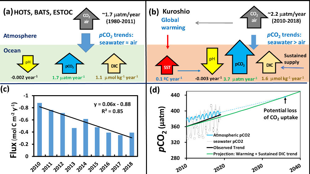
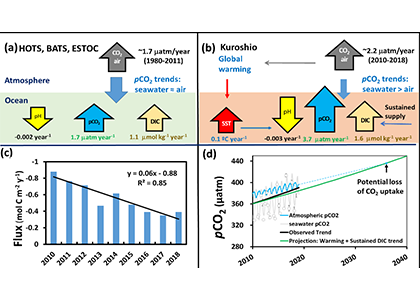
Figure 1. Graphic summary of 9 years of data from the Kuroshio Current time-series: (a) under the influences of only atmospheric CO2 increase, (b) the combined effect of atmospheric CO2 increase, SST increase, and additional DIC supply, (c) annually averaged air-sea CO2 flux decrease, (d) Projected seawater pCO2 increase under SST rise and sustained DIC increase.
A recent study in Marine Pollution Bulletin documented the rapid increase of seawater pCO2 (3.70±0.57 matm year-1) and acidification (pH at -0.0033±0.0009 unit year-1) along Kuroshio in the East China Sea (Figure 1). These findings were based on nine years of time-series data ( 2010-2018) which are now available on the website of Japan Meteorological Agency (JMA). These trends are significantly greater than the expected rates from CO2 air-sea equilibrium and those reported from other oceanic time-series studies. Interestingly, they showed the contribution of each parameter such as sea surface temperature (SST), sea surface salinity (SSS), and normalized dissolved inorganic carbon (nDIC) and total alkalinity (nTA) to the pCO2 variability. Seawater warming caused rapid rates of pCO2 increase and acidification under sustained DIC increase. The faster pCO2 growth relative to the atmosphere resulted in the CO2 uptake through the air-sea exchange declining by ~50% (~-0.8 to -0.4 mol C m-2 y-1) over the study period.
If this trend continues and the atmospheric CO2 increases at its current rate, the rapid warming Kuroshio regions could change from a sink to a source of CO2 , and cause a loss of oceanic CO2 uptake in the near future (ca. 2030-2040). Further, other “warming hotspots” in the global ocean along western boundary currents with a continuous DIC supply may exhibit similarly accelerated acidification and pCO2 rise. This could lead to a significant reduction in ocean CO2 uptake.
Authors:
Shou-En Tsao (Institute of Oceanography, National Taiwan University, Taiwan)
Po-Yen Shen (Institute of Oceanography, National Taiwan University, Taiwan)
Chun-Mao Tseng* (Institute of Oceanography, National Taiwan University, Taiwan)