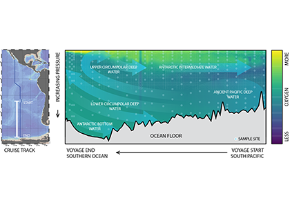
Global overturning circulation is a planetary conveyor belt: dense waters sink around Antarctica, spread through the deep ocean for centuries, and eventually rise elsewhere, redistributing heat, nutrients, and carbon. But how does this slow, pervasive movement of water impact marine microbes?
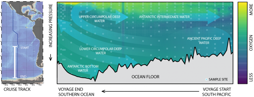
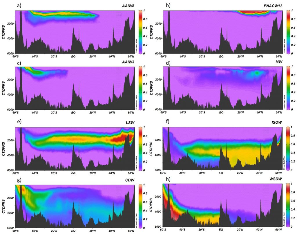
To find out, researchers collected over 300 water samples spanning the full depth of the ocean along the GO-SHIP P18 line in the South Pacific. They found that microbial genomes cluster into six spatial cohorts that are not only delineated by depth, but also circulatory features, like Antarctic Bottom Water formation, and ventilation age. Distinct functional signatures also emerged across these circulation-driven zones. For example, genes for light harvesting and iron uptake dominate in surface waters, while adaptations for cold, high pressure, or anaerobic metabolism characterize deep and ancient waters. Antarctic Bottom Water communities also carry hallmarks of rapid genetic exchange, suggesting horizontal gene transfer may help microbes adapt as they sink into the deep ocean. Even in waters isolated from the atmosphere for over a thousand years, many microbial genomes have coverage patterns that imply active replication, demonstrating that long-isolated water masses still support active microbial populations. In considering patterns of microbial diversity, researchers also identified a pervasive “prokaryotic phylocline” in which richness spikes just below the surface mixed layer and remains high to full ocean depth, only dipping slightly in very old water.
These results demonstrate that physical circulation, not just temperature or nutrients, partitions the ocean into microbial biomes. Understanding this linkage is critical because microbes determine the amount of carbon that is recycled or stored long-term in the deep ocean. As climate change alters overturning circulation, the functioning of these hidden microbial ecosystems and their role in regulating atmospheric CO₂ may shift in unexpected ways.
Authors
Bethany C. Kolody (University of California San Diego; UC Berkeley; J. Craig Venter Institute)
Rohan Sachdeva (UC Berkeley)
Hong Zheng (J. Craig Venter Institute)
Zoltán Füssy (UC San Diego; J. Craig Venter Institute)
Eunice Tsang (UC Berkeley)
Rolf E. Sonnerup (University of Washington)
Sarah G. Purkey (UC San Diego)
Eric E. Allen (UC San Diego)
Jillian F. Banfield (UC Berkeley; Lawrence Berkeley National Laboratory; Monash University)
Andrew E. Allen (UC San Diego; JCVI)
Social media
Twitter/X: @science_doodles, @Scripps_Ocean, @JCVenterInst
Bluesky: @banfieldlab.bsky.social, @bethanykolody.bsky.social, @scrippsocean.bsky.social, @jcvi.org
https://www.science.org/doi/10.1126/science.adv6903
Overturning circulation structures the microbial functional seascape of the South Pacific
Science