Ocean Carbon & Biogeochemistry
Studying marine ecosystems and biogeochemical cycles in the face of environmental change
  • Home
  • About OCB
    • About Us
    • Scientific Breadth
      • Biological Pump
      • Changing Marine Ecosystems
      • Changing Ocean Chemistry
      • Estuarine and Coastal Carbon Fluxes
      • Ocean Carbon Uptake and Storage
      • Ocean Observatories
    • Code of Conduct
    • Get Involved
    • Project Office
    • Scientific Steering Committee
    • OCB committees
      • Ocean Time-series
      • US Biogeochemical-Argo
      • Ocean-Atmosphere Interaction
  • Activities
    • Summer Workshop
    • OCB Webinars
    • Guidelines for OCB Workshops & Activities
    • Topical Workshops
      • CMIP6 Models Workshop
      • Coastal BGS Obs with Fisheries
      • C-saw extreme events workshop
      • Expansion of BGC-Argo and Profiling Floats
      • Fish, fisheries and carbon
      • Future BioGeoSCAPES program
      • GO-BCG Scoping Workshop
      • Lateral Carbon Flux in Tidal Wetlands
      • Leaky Deltas Workshop – Spring 2025
      • Marine CDR Workshop
      • Ocean Nucleic Acids ‘Omics
      • Pathways Connecting Climate Changes to the Deep Ocean
    • Small Group Activities
      • Aquatic Continuum OCB-NACP Focus Group
      • Arctic-COLORS Data Synthesis
      • BECS Benthic Ecosystem and Carbon Synthesis WG
      • Carbon Isotopes in the Ocean Workshop
      • CMIP6 WG
      • Filling the gaps air–sea carbon fluxes WG
      • Fish Carbon WG
      • Meta-eukomics WG
      • mCDR
      • Metaproteomic Intercomparison
      • Mixotrophs & Mixotrophy WG
      • N-Fixation WG
      • Ocean Carbonate System Intercomparison Forum
      • Ocean Carbon Uptake WG
      • OOI BGC sensor WG
      • Operational Phytoplankton Observations WG
      • Phytoplankton Taxonomy WG
    • Other Workshops
    • Science Planning
      • Coastal CARbon Synthesis (CCARS)
      • North Atlantic-Arctic
    • Ocean Acidification PI Meetings
    • Training Activities
      • PACE Hackweek 2025
      • PACE Hackweek 2024
      • PACE Training Activity 2022
  • Science Support
    • Data management and archival
    • Early Career
    • Funding Sources
    • Jobs & Postdocs
    • Meeting List
    • OCB Topical Websites
      • Ocean Fertilization
      • Trace gases
      • US IIOE-2
    • Outreach & Education
    • Promoting your science
    • Student Opportunities
    • OCB Activity Proposal Solicitations
      • Guidelines for OCB Workshops & Activities
    • Travel Support
  • Publications
    • OCB Workshop Reports
    • Science Planning and Policy
    • Newsletter Archive
  • Science Highlights
  • News

Archive for food webs – Page 3

Phytoplankton can actively diversify their migration strategy in response to turbulent cues

Posted by mmaheigan 
· Thursday, August 17th, 2017 

Turbulence is known to be a primary determinant of plankton fitness and succession. However, open questions remain about whether phytoplankton can actively respond to turbulence and, if so, how rapidly they can adapt to it. Recent experiments have revealed that phytoplankton can behaviorally respond to turbulent cues with a rapid change in shape, and this response occurs over a few minutes. This challenges a fundamental paradigm in oceanography that phytoplankton are passively at the mercy of turbulence.

Phytoplankton are photosynthetic microorganisms that form the base of most aquatic food webs, impact global biogeochemical cycles, and produce half of the world’s oxygen. Many species of phytoplankton are motile and migrate in response to gravity and light levels: Upward toward light during the day to photosynthesize and downward at night toward higher nutrient concentrations. Disruption of this diurnal migratory strategy is an important contributor to the succession between motile and non-motile species when conditions become more turbulent. However, this classical view neglects the possibility that motile species can actively respond in an effort to avoid layers of strong turbulence. A recent study by Sengupta, Carrara and Stocker, published in Nature has shown that some raphidophyte and dinoflagellate phytoplankton can actively diversify their migratory strategy in response to hydrodynamic cues characteristic of overturning by the smallest turbulent eddies in the ocean. Laboratory experiments in which cells experienced repeated overturning with timescales and statistics representative of ocean turbulence revealed that over timescales as short as ten minutes, an upward-swimming population split into two subpopulations, one swimming upward and one swimming downward. Quantitative morphological analysis of the harmful algal bloom-forming raphidophyte Heterosigma akashiwo revealed that this behavior was accompanied by a change in cell shape, wherein the cells that changed their swimming direction did so by going from an asymmetric pear shape to a more symmetric egg shape. A model of cell mechanics showed that the magnitude of this shift was minute, yet sufficient to invert the cells’ preferential swimming direction. The results highlight the advanced level of control that phytoplankton have on their migratory behavior.

Understanding how fluctuations in the oceans’ turbulence landscape impacts phytoplankton is of fundamental importance, especially for predicting species succession and community structure given projected climate-driven changes in temperature, winds, and upper ocean structure.

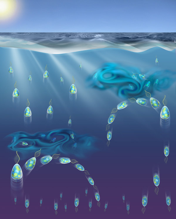
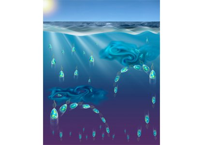
An upward-swimming phytoplankton population splits into upward- and downward-swimming sub-populations when exposed to turbulent eddies, due to a subtle change in cell shape. Illustration by: A. Sengupta, G. Gorick, F. Carrara and R. Stocker


This work was co-funded by a Human Frontier Science Program Cross Disciplinary Fellowship (LT000993/2014-C to A.S.), a Swiss National Science Foundation Early Postdoc Mobility Fellowship (to F.C.), and a Gordon and Betty Moore Marine Microbial Initiative Investigator Award (GBMF 3783 to R.S.)


International team of researchers reports ocean acidification is spreading rapidly in the western Arctic Ocean

Posted by mmaheigan 
· Thursday, March 30th, 2017 

The Arctic Ocean is particularly sensitive to climate change and ocean acidification such that aragonite saturation state is expected to become undersaturated (Ωarag <1) there sooner than in other oceans. However, the extent and expansion rate of ocean acidification (OA) in this region are still unknown.

In the March 2017 issue of Nature Climate Change, Qi et al. show that, between 1994 and 2010, low Ωarag waters have expanded northwards at least 5º, to 85ºN, and deepened from 100 m to 250 m depth. Data from multiple trans-western Arctic Ocean cruises show that Ωarag<1 water has increased in the upper 250 m from 5 to 31% of the total area north of 70ºN. Tracer data and model simulations suggest that increased transport of Pacific Winter Water (which is already acidified due to both natural and anthropogenic sources), driven by sea-ice retreat and the circulation changes, are primarily responsible for the expansion, while local carbon recycling and anthropogenic CO2 uptake have also contributed. These results indicate more rapid acidification is occurring in the Arctic Ocean, two to four times faster than the Pacific and Atlantic Oceans, with the western Arctic Ocean the first open-ocean region with large-scale expansion of “acidified” water directly observed in the upper water column.

The rapid spread of ocean acidification in the western Arctic has implications for marine life, particularly clams, mussels and pteropods that may have difficulty building or maintaining their shells in increasingly acidified waters. The pteropods are part of the Arctic food web and important to the diet of salmon and herring. Their decline could affect the larger marine ecosystem.

Authors:
Richard A. Feely (NOAA Pacific Marine Environmental Laboratory)
Leif G. Anderson (Univ. of Gothenburg)
Heng Sun (SOA Third Institute of Oceanography)
Jianfang Chen (SOA Second Institute of Oceanography
Min Chen (Univ. of Delaware)
Liyang Zhan (SOA Third Institute of Oceanography)
Yuanhui Zhang (SOA Third Institute of Oceanography)
Wei-Jun Cai (Univ. of Delaware, Univ. of Georgia)

Reconciling fisheries catch and ocean productivity in a changing climate

Posted by mmaheigan 
· Thursday, March 16th, 2017 

Phytoplankton provide the energy that fuels marine food webs, yet differences in fisheries catch across global ecosystems far exceed accompanying differences in phytoplankton production. Nearly 50 years ago, John Ryther hypothesized that this contrast must arise from synergistic interactions between phytoplankton production and food webs. New perspectives on global fish catch, fishing effort, and a prototype high-resolution global earth system model allowed us to revisit Ryther’s supposition and explore its implications under climate change. After accounting for a small number of lightly fished ecosystems, we find that stark differences in regional catch can be explained with an energetically constrained model that a) resolves large inter-regional differences in the benthic and pelagic energy pathways connecting phytoplankton and fish; b) reduces trophic transfer efficiencies in warm, tropical ecosystems; and, less critically, c) associates elevated trophic transfer efficiencies with benthic systems. The same food web processes that accentuate spatial differences in phytoplankton production in the contemporary ocean also accentuated temporal trends under climate change, with projected fish catch changes in some areas exceeding 50% (Figure 1). Our results, recently published in PNAS, demonstrate the importance of marine resource management strategies that are robust to potentially significant changes in fisheries productivity baselines. These results also provide impetus for efforts to improve constraints on regional ocean productivity projections that often disagree in present earth system models.

Figure 1: Projected percent changes in net phytoplankton production (left) and fisheries catch (right) between 2050-2100 and 1950-2000 under a high greenhouse gas emission scenario (RCP8.5) in GFDL’s ESM2M-COBALT Earth System Model. Contours are shown for +/- 50%.


Authors: Charles A. Stocka, Jasmin G. Johna, Ryan R. Rykaczewskib,c, Rebecca G. Aschd, William W.L. Cheunge, John P. Dunnea, Kevin D. Friedlandf, Vicky W.Y. Lame, Jorge L. Sarmientod, and Reg A. Watsong

aGeophysical Fluid Dynamics Laboratory, National Oceanic and Atmospheric Administration 
bSchool of the Earth, Ocean, and Environment, University of South Carolina 
cDepartment of Biological Sciences, University of South Carolina
dAtmospheric and Oceanic Sciences Program, Princeton University
eNippon Foundation-Nereus Program, Institute of Oceans and Fisheries, The University of British Columbia
fNational Marine Fisheries Service, Narragansett, RI
gInstitute for Marine and Antarctic Studies, University of Tasmania, Australia

ENSO impacts on ecosystem indicators in the California Current System

Posted by mmaheigan 
· Thursday, February 16th, 2017 

El Niño-Southern Oscillation (ENSO) events activate long-distance teleconnections through the atmosphere and ocean that can dramatically impact marine ecosystems along the West Coast of North America, affecting diverse organisms ranging from plankton to exploitable and protected species. Such ENSO-related changes to marine ecosystems can ultimately affect humans in many ways, including via depressed plankton and fish production, dramatic range shifts for many protected and exploited species, inaccessibility of traditionally fished resources, more prevalent harmful algal blooms, altered oxygen and pH of waters used in mariculture, and proliferation of pathogens. The principal objective of the Forecasting ENSO Impacts on Marine Ecosystems of the US West Coast workshop was to develop a scientific framework for building an ENSO-related forecast system of ecosystem indicators along the West Coast of North America, including major biological and biogeochemical responses. Attendees realized that a quantitative, biologically-focused forecast system is a much more challenging objective than forecasting the physical system alone; it requires an understanding of the ocean-atmospheric physical system and of diverse organism-level, population-level, and geochemical responses that, in aggregate, lead to altered ecosystem states.

In the tropical ocean, important advances have been made in developing both intensive observational infrastructure (Global Tropical Moored Buoy Array) and diverse dynamical and statistical models that utilize these data in ENSO forecasting. These forecasts are made widely available (e.g., NOAA’s Climate Prediction Center). The most sophisticated ENSO-forecasting efforts use global, coupled ocean-atmosphere climate models that extend ENSO-forecasting skill into seasonal climate forecasting skill for other regions, including the California Current System (CCS). However, both these measurement systems and forecast models are restricted to the physical dynamics of ENSO, rather than biotic and biogeochemical consequences.

Primary modes of influence of El Niño on marine organisms

In this brief discussion, we focus primarily on the warm (El Niño) phases of ENSO, which can have large and generally negative ecosystem consequences, although changes accompanying the cold phases (La Niña) can also be significant. We primarily address pelagic ocean processes, which merely reflect the expertise of the participants at the workshop. Physical mechanisms by which ENSO impacts the U.S. West Coast are more completely explained in Jacox et al. (this issue).

El Niño affects organisms and biogeochemistry via both local and advective processes (Figure 1). ENSO-related changes in the tropics can affect the CCS through an atmospheric teleconnection (Alexander et al. 2002) to alter local winds and surface heat fluxes, and through upper ocean processes (thermocline and sea level displacements and geostrophic currents) forced remotely by poleward propagating coastally trapped waves (CTWs) of tropical origin (Enfield and Allen 1980; Frischkencht et al. 2015; Figure 1). It is important to recognize that ecosystem effects will occur through three primary mechanisms: (1) via the direct action of altered properties like temperature, dissolved O2, and pH on the physiology and growth of marine organisms; (2) through food web effects as changes in successive trophic levels affect their predators (bottom up) or prey (top down); and (3) through changes in advection related to the combination of locally forced Ekman transport and remotely forced geostrophic currents, typically involving poleward and/or onshore transport of organisms. Advective effects can be pronounced, transporting exotic organisms into new regions and altering the food web if these imported species have significant impacts as predators, prey, competitors, parasites, or pathogens.

Figure 1. Schematic illustration of dominant mechanisms through which ENSO impacts biological and biogeochemical processes in the California Current System. Processes include both local effects (e.g., heat budget, winds) and advective effects. Such processes can influence organisms via: (1) (yellow arrow) direct physiological responses to changes in temperature, O2, pH, etc.; (2) (orange arrows) effects that propagate through the food web, as successive trophic levels affect their predators (bottom up, upward-facing orange arrows) or prey (top down, downward-facing orange arrows); (3) (blue arrows) direct transport effects of advection. Top predators are not included here. CTW indicates coastally trapped waves.


I. Poleward and onshore transport

Active, mobile marine fishes, seabirds, reptiles, and mammals may move into new (or away from old) habitats in the CCS as ENSO-related changes occur in the water column and render the physical-chemical characteristics and prey fields more (or less) suitable for them. Planktonic organisms are often critical prey and are, by definition, subject to geographic displacements as a consequence of altered ocean circulation that accompanies El Niño events. Most commonly, lower latitude organisms are transported poleward to higher latitudes in either surface flows or in an intensified California Undercurrent (Lynn and Bograd 2002). However, some El Niño events are accompanied by onshore flows (Simpson 1984), potentially displacing offshore organisms toward shore (Keister et al. 2005).

Two of the most celebrated examples of poleward transport come from distributions of pelagic red crabs (Pleuroncodes planipes) and the subtropical euphausiid (or krill, Nyctiphanes simplex), both of which have their primary breeding populations in waters off Baja California, Mexico (Boyd 1967; Brinton et al. 1999). Pelagic red crabs were displaced approximately 10° of latitude, from near Bahia Magdalena, Baja California, northward to Monterey, California (Glynn 1961; Longhurst 1967) during the El Niño of 1958-1959. This early event was particularly well documented because of the broad latitudinal coverage of the California Cooperative Oceanic Fisheries Investigations (CalCOFI) cruises at the time. Such El Niño-related northward displacements have been documented repeatedly over the past six decades (McClatchie et al. 2016), partly because the red crabs often strand in large windrows on beaches and are conspicuous to the general public. The normal range of the euphausiid Nyctiphanes simplex is centered at 25-30°N (Brinton et al. 1999). N. simplex has been repeatedly detected far to the north of this range during El Niño, extending at least to Cape Mendocino (40.4°N) in 1958 (Brinton 1960), to northern Oregon (46.0°N) in 1983 (Brodeur 1986), and to Newport, Oregon (44.6°N; Keister et al. 2005) and northwest Vancouver Island (50.7°N; Mackas and Galbraith 2002) in 1998. In spring of 2016, N. simplex were extremely abundant in the southern California region (M. Ohman and L. Sala, personal communication) and detected as far north as Trinidad Head (41.0°N) but not in Newport, Oregon (W. Peterson, personal communication). Sometimes such El Niño-related occurrences of subtropical species are accompanied by declines in more boreal species (e.g., Mackas and Galbraith 2002; Peterson et al. 2002), although this is not always the case.

Among the organisms displaced during El Niños, the consequences of transport of predators are poorly understood but likely significant in altering the food web.  Subtropical fishes can be anomalously abundant in higher latitudes during El Niño (Hubbs 1948; Lluch-Belda et al. 2005; Pearcy and Schoener 1987; Pearcy 2002; Brodeur et al. 2006), with significant consequences for the resident food web via selective predation on prey populations.

II. Habitat compression

Many species are confined to a specific habitat that may compress during El Niño. This phenomenon has been observed repeatedly for species and processes related to coastal upwelling in the CCS. During major El Niño events, as the offshore extent of upwelled waters is reduced and becomes confined close to the coast, the zone of elevated phytoplankton (observed as Chl-a) compresses markedly to a narrow zone along the coastal boundary (e.g., Kahru and Mitchell 2000; Chavez et al. 2002). For example, during the strong El Niño spring of 1983, the temperate euphausiid Euphausia pacifica was present in low densities throughout Central and Southern California waters, but 99% of the biomass was unusually concentrated at a single location (station 80.51) very close to Point Conception, where upwelling was still pronounced (E. Brinton, personal communication). The spawning habitat of the Pacific sardine (Sardinops sagax) was narrowly restricted to the coastal boundary during El Niño 1998, but one year later during La Niña 1999, the spawning habitat extended a few hundred kilometers farther offshore (Lo et al. 2005). Market squid, Doryteuthis opalescens, show dramatically lower catches during El Niño years (Reiss et al. 2004), but in 1998, most of the catch was confined to a small region in Central California (Reiss et al. 2004). During the El Niño in spring 2016, vertical particle fluxes measured by sediment traps were reduced far offshore but remained elevated in the narrow zone of coastal upwelling very close to Point Conception (M. Stukel, personal communication).

III. Altered winds and coastal upwelling

Upwelling-favorable winds along the US West Coast may decline during El Niño conditions (Hayward 2000, but see Chavez et al. 2002) and vertical transports can be reduced (Jacox et al. 2015), mainly during the winter and early spring (Black et al. 2011). Independent of any changes in density stratification (considered below), these decreased vertical velocities can lead to diminished nutrient fluxes, reduced rates of primary production, and a shift in the size composition of the plankton community to smaller phytoplankton and zooplankton (Rykaczewski and Checkley 2008). Such changes at the base of the food web can have major consequences for a sequence of consumers at higher trophic levels, as both the concentration and suitability of prey decline.

However, there are potential compensatory effects of reduced rates of upwelling. Diminished upwelling also means less introduction of CO2-rich, low-oxygen waters to coastal areas (Feely et al. 2008; Bednaršek et al. 2014), with potential benefits to organisms that are sensitive to calcium carbonate saturation state or hypoxic conditions. Furthermore, reduced upwelling implies lower Ekman transport and potentially reduced cross-shore fluxes far offshore within coastal jets and filaments (cf., Keister al. 2009).

IV. Increased stratification and deepening of nutricline

El Niño-related warming of surface waters and increased density stratification can result from advection of warmer waters and/or altered local heating. Evidence suggests that the pycnocline (Jacox et al. 2015) and nitracline (Chavez et al. 2002) deepen during stronger El Niños. This effect, independent of variations in wind stress, also leads to diminished vertical fluxes of nitrate and other limiting nutrients and suppressed rates of primary production. Decreased nitrate fluxes appear to explain elevated 15N in California Current zooplankton (Ohman et al. 2012) and decreased krill abundance (Lavaniegos and Ohman 2007; Garcia-Reyes et al. 2014) during El Niño years. For example, the 2015-16 El Niño resulted in a pronounced warming of surface waters and depressed Chl-a concentrations across a broad region of the CCS (McClatchie et al. 2016).

V. Direct physiological responses to altered temperature, dissolved O2, pH

Most organisms in the ocean—apart from some marine vertebrates—are ectothermic, meaning they have no capability to regulate their internal body temperature. Heating or cooling of the ocean therefore directly influences their rates of metabolism, growth, and mortality. Most organisms show not only high sensitivity to temperature variations but nonlinear responses. A typical temperature response curve or “thermal reaction norm” (e.g., of growth rate) is initially steeply positive with increasing temperature, followed by a narrow plateau, then abruptly declines with further increases in temperature (e.g., Eppley 1972). Different species often show different thermal reaction norms. Hence, El Niño-related temperature changes may not only alter the growth rates and abundances of organisms, but also shift the species composition of the community due to differential temperature sensitivities.

Similarly, El Niño-induced variations in dissolved oxygen concentration and pH can have marked consequences for physiological responses of planktonic and sessile benthic organisms and, for active organisms, potentially lead to migrations into or out of a suitable habitat. Interactions between variables (Boyd et al. 2010) will also lead to both winners and losers in response to major ENSO-related perturbations.

Altered parasite, predator populations, and harmful algal blooms

ENSO-related changes can favor the in situ proliferation or introduction of predators, parasites, pathogens, and harmful algal blooms. Such outbreaks can have major consequences for marine ecosystems, although some are relatively poorly studied. For example, a recent outbreak of sea star wasting disease thought to be caused by a densovirus adversely affected sea star populations at numerous locations along the West Coast (Hewson et al. 2014). While not specifically linked to El Niño, this outbreak was likely tied to warmer water temperatures. Because some sea stars are keystone predators capable of dramatically restructuring benthic communities (Paine 1966), such pathogen outbreaks are of considerable concern well beyond the sea stars themselves.

Domoic acid outbreaks, produced by some species of the diatom genus Pseudo-nitzschia, can result in closures of fisheries for razor clams, Dungeness crab, rock crab, mussels, and lobsters, resulting in significant economic losses. While the causal mechanisms leading to domoic outbreaks are under discussion (e.g., Sun et al. 2011; McCabe et al. 2016), warmer-than-normal ocean conditions in northern regions of the CCS have been linked to domoic acid accumulation in razor clams, especially when El Niño conditions coincide with the warm phase of the Pacific Decadal Oscillation (McKibben et al. 2017).

ENSO diversity, non-stationarity, and consequences of secular changes

There is considerable interest in understanding the underlying dynamical drivers that lead to different El Niño events (Singh et al. 2011; Capotondi et al. 2015). Although there appears to be a continuum of El Niño expression along the equatorial Pacific, some simplify this continuum to a dichotomy between Eastern Pacific (EP) and Central Pacific (CP) events (Capotondi et al 2015). Whether EP and CP El Niños have different consequences for mid-latitude ecosystems like the California Current Ecosystem is an area of open research, but some evidence suggests that differences in timing and intensity of biological effects may exist (cf. Fisher et al. 2015). While some studies (e.g., Lee and McPhaden 2010) suggest that the frequency of CP El Niños is increasing, the evidence is not definitive (Newman et al. 2011). In addition to questions about the ecosystem consequences of El Niño diversity, there are unknowns regarding interactions between El Niño, decadal-scale variability (Chavez et al. 2002), and secular changes in climate (Figure 2, Ohman, unpubl.), which suggest a non-stationary relationship between California Current zooplankton and El Niño. An index of the dominance of warm water krill from CalCOFI sampling in Southern California shows that for the first 50 years there was a predictable positive relationship between these warm water krill and El Niño. This relationship held during both EP and CP El Niño events from 1950-2000. However, the relationship appeared to weaken after 2000. The warm water krill index was negatively correlated with the moderate El Niño of 2009-10. While the krill index again responded to the major El Niño of 2015-16 and the preceding year of warm anomalies (Bond et al. 2015; Zaba and Rudnick 2016), the magnitude of the response was not comparable to what had been seen in earlier decades. It is unclear whether such results are merely the consequence of interannual variability in the mode of El Niño propagation (Todd et al. 2011) or a change in the relationship between El Niño forcing and ecosystem responses.


Figure 2. Covariability of California Current euphausiids (krill, blue lines) with an index of ENSO off California (de-trended sea level anomaly [DTSLA] at San Diego, green lines). Note the markedly different relationship between euphausiids and DTSLA after 2000. Sustained excursions of DTSLA exceeding one standard deviation (i.e., above upper dotted red line) are expressions of El Niño (or of the warm anomaly of 2014-2015). Red arrows indicate specific events categorized as either eastern Pacific (EP) or central Pacific (CP) El Niño events (Yu et al. 2012), apart from 2015-2016 which could be either CP or EP. The Warm-Cool euphausiid index is based on the difference in average log carbon biomass anomaly of the four dominant warm water euphausiids in the CCS minus the average anomaly of the four dominant cool water euphausiids (species affinities from Brinton and Townsend 2003). Euphausiid carbon biomass from springtime CalCOFI cruises off Southern California, lines 77-93, nighttime samples only. Dotted blue lines indicate years of no samples (Ohman, personal communication).

Conclusions

While the potential modes of El Niño influence on biological and biogeochemical processes in the CCS are numerous, not all processes are of first order consequence to all organisms. Forecasting ENSO effects on a given target species will likely focus on a limited number of governing processes. Table 1 illustrates some of the specific types of organisms susceptible to El Niño perturbations and the suspected dominant mechanism. We look forward to developing a framework for forecasting such responses in a quantitative manner.

Ecosystem indicator Region and season Change during El Niño Time scale of response Regional ocean processes
Primary production Entire CCS

winter, spring, summer

Declines Variable lag;

Instantaneous or time-lagged

Reduced upwelling, nutrient fluxes; Deeper nutricline and weaker winds
Pseudo-nitzschia diatoms; Domoic Acid Entire CCS

spring-summer

Blooms  

1-3 month lag

Elevated temperature; Altered nutrient stoichiometry
Copepod assemblage NCCS

spring-summer

Warm water species appear Nearly instantaneous Poleward advection; Reduced upwelling, warmer temperature
 

Subtropical euphausiids


SCCS

spring-summer


Increase

Nearly instantaneous; persists beyond Niño event Poleward advection
Cool water euphausiids Entire CCS

spring-summer

Decrease Time-lagged Reduced upwelling; Anomalous advection
Pelagic red crabs SCCS & CCCS

winter, spring, summer

Increase Nearly instantaneous Poleward advection
Market squid CCCS & SCCS

winter & spring

Collapse Instantaneous for distribution; time-lagged for recruitment Warmer temperature/deeper thermocline; Reduces spawning habitat
Pacific sardine Entire CCS

winter-spring

Changes in distribution;

Compression of spawning habitat

Instantaneous for spawning and distribution, recruitment time-lagged, biomass is time-integrated Wind stress, cross-shore transport


Northern anchovy CCCS & SCCS

winter-spring

Changes in distribution;

Compression of spawning habitat

Instantaneous for spawning and distribution, recruitment time-lagged, biomass is time-integrated Reduced upwelling; Anomalous advection


Juvenile salmon survival NCCS

spring-summer

Decrease in Pacific NW Time-integrated Reduce river flow, decreased food supply in ocean
Adult sockeye salmon

(Fraser River)

NCCS

summer

Return path deflected northward to Canadian waters Time-integrated Ocean temperature, including Ekman controls
Warm assemblage of mesopelagic fish SCCS

spring (?)

Increase Lagged 0-3 months Poleward and onshore advection
Common murre

(reproductive success)

CCCS

winter-spring

Decrease Time-Lagged, time-integrated Prey (fish) availability; Thermocline depth; Decreased upwelling?
Top predator reproduction and abundance Entire CCS Species-dependent Time-integrated Advection of prey, altered temperature, upwelling, mesoscale structure
Top predator distribution Entire CCS Altered geographic distributions Instantaneous or time-lagged Advection of prey, altered temperature, upwelling, mesoscale structure
Table 1.   Examples of water column biological processes and organisms known to be affected by El Niño in the California Current System. Columns indicate the type of organism; approximate geographic region and season of the effect; direction of change in response to El Niño; temporal pattern of response (immediate, time-lagged, time-integrated); and the hypothesized oceanographic processes driving the organism response. CCS = California Current System; NCCS, CCCS, and SCCS denote northern, central, and southern sectors of the CCS.


Authors

Mark D. Ohman (Scripps Institution of Oceanography)
Nate Mantua (NOAA Southwest Fisheries Science Center)
Julie Keister (University of Washington)
Marisol Garcia-Reyes (Farallon Institute)
Sam McClatchie (NOAA Southwest Fisheries Science Center)

References

Alexander, M. A., I. Blade, M. Newman, J. R. Lanzante, N. C. Lau, and J. D. Scott, 2002: The atmospheric bridge: The influence of ENSO teleconnections on air-sea interaction over the global oceans. Journal of Climate, 15, 2205-2231, doi: 10.1175/1520-0442(2002)015<2205:TABTIO>2.0.CO;2

Bednaršek, N., R. A. Feely, J. C. P. Reum, B. Peterson, J. Menkel, S. R. Alin, and B. Hales, 2014: Limacina helicina shell dissolution as an indicator of declining habitat suitability owing to ocean acidification in the California Current Ecosystem. Proc. Roy. Soc. B-Biolog. Sci., 281, doi: 10.1098/rspb.2014.0123.

Black, B. A., I. D. Schroeder, W. J. Sydeman, S. J. Bograd, B. K. Wells, and F. B. Schwing, 2011: Winter and summer upwelling modes and their biological importance in the California Current Ecosystem. Glob. Change Bio., 17, 2536-2545, doi: 10.1111/j.1365-2486.2011.02422.x.

Bond, N. A., M. F. Cronin, H. Freeland, and N. Mantua, 2015: Causes and impacts of the 2014 warm anomaly in the NE Pacific. Geophy. Res. Lett., 42, 3414-3420, doi: 10.1002/2015GL063306.

Boyd, C. M., 1967: The benthic and pelagic habitats of the red crab, Pleuroncodes planipes. Pacific Science, 21, 394-403.

Boyd, P. W., R. Strzepek, F. X. Fu, and D. A. Hutchins, 2010: Environmental control of open-ocean phytoplankton groups: Now and in the future. Limnol. Oceanogr., 55, 1353-1376, doi: 10.4319/lo.2010.55.3.1353.

Brinton, E., 1960: Changes in the distribution of euphausiid crustaceans in the region of the California Current. CalCOFI Reports, 7, 137-146, http://www.calcofi.org/publications/calcofireports/v07/Vol_07_Brinton.pdf.

Brinton, E., M. D. Ohman, A. W. Townsend, M. D. Knight, and A. L. Bridgeman, 1999: Euphausiids of the World Ocean. Vol. CD-ROM, MacIntosh version 1.0, UNESCO Publishing.

Brodeur, R. D., 1986: Northward displacement of the euphausiid Nyctiphanes simplex Hansen to Oregon and Washington waters following the El Niño event of 1982-83. J. Crustacean Bio., 6, 686-692, doi: 10.2307/1548382.

Brodeur, R. D., S. Ralston, R. L. Emmett, M. Trudel, T. D. Auth, and A. J. Phillips, 2006: Anomalous pelagic nekton abundance, distribution, and apparent recruitment in the northern California Current in 2004 and 2005. Geophy. Res. Lett., 33, doi:10.1029/2006gl026614.

Capotondi, A., and Coauthors, 2015: Understanding ENSO Diversity. Bull. Amer. Meteor. Soc., 96, 921-938, doi: 10.1175/BAMS-D-13-00117.1.

Chavez, F. P., and Coauthors, 2002: Biological and chemical consequences of the 1997–1998 El Niño in central California waters. Prog. Oceanogr., 54, 205-232, doi: 10.1016/S0079-6611(02)00050-2.

Enfield, D., and J. Allen, 1980: On the structure and dynamics of monthly mean sea-level anomalies along the Pacific coast of North and South America. J. Phys. Oceanogr., 10, 557–578, doi: 10.1175/1520-0485(1980)010<0557:OTSADO>2.0.CO;2.

Eppley, R. W., 1972: Temperature and phytoplankton growth in the sea. Fish. Bull, 70, 1063-1085, http://fishbull.noaa.gov/70-4/eppley.pdf.

Feely, R. A., C. L. Sabine, J. M. Hernandez-Ayon, and D. H. Ianson, B., 2008: Evidence for upwelling of corrosive “acidified” water onto the continental shelf. Science, 320, 1490-1492, doi: 10.1126/science.1155676.

Fisher J. L., W. T. Peterson, and R. R. Rykaczewski, 2015: The impact of El Niño events on the pelagic food chain in the northern California Current. Glob. Change Bio., 21, 4401–4414, doi: 10.1111/gcb.13054.

Frischknecht, M., M. Münnich, and N. Gruber, 2015: Remote versus local influence of ENSO on the California Current System, J. Geophys. Res. Oceans, 120, 1353–1374, doi:10.1002/2014JC010531.

García-Reyes, M., J. L. Largier, and W. J. Sydeman, 2014: Synoptic-scale upwelling indices and predictions of phyto-and zooplankton populations. Prog. Oceanogr., 120, 177-188, doi: 10.1016/j.pocean.2013.08.004.

Glynn, P. W., 1961: The first recorded mass stranding of pelagic red crabs, Pleuroncodes planipes, at Monterey Bay, California, since 1859, with notes on their biology. Cal. Fish Game, 47, 97-101.

Hayward, T. L., 2000: El Niño 1997-98 in the coastal waters of Southern California: a timeline of events. CalCOFI Reports, 41, 98-116, http://www.calcofi.org/publications/calcofireports/v41/Vol_41_Hayward.pdf.

Hewson, I., and Coauthors, 2014: Densovirus associated with sea-star wasting disease and mass mortality. Proc. Nat. Acad. Sci., 111, 17278-17283, doi: 0.1073/pnas.1416625111.

Hubbs, C. L., 1948: Changes in the fish fauna of western North America correlated with changes in ocean temperature, J. Mar. Res., 7, 459– 482, http://www.nativefishlab.net/library/textpdf/20041.pdf.

Jacox, M. G., J. Fiechter, A. M. Moore, and C. A. Edwards, 2015: ENSO and the California Current coastal upwelling response. J. Geophy. Res. Oceans, 120, 1691-1702, doi: 10.1002/2014JC010650.

Jacox, M.G. …..   [this issue of Variations]  PLEASE ADD FULL REFERENCE

Kahru, M., E. Di Lorenzo, M. Manzano-Sarabia, and B. G. Mitchell, 2012: Spatial and temporal statistics of sea surface temperature and chlorophyll fronts in the California Current. J. Plank. Res., 34, 749-760, doi: 10.1093/plankt/fbs010.

Kahru, M., and B. G. Mitchell, 2000: Influence of the 1997-98 El Niño on the surface chlorophyll in the California Current. Geophys.Res.Lett., 27, 2937-2940, doi: 10.1029/2000GL011486

Keister, J. E., T. J. Cowles, W. T. Peterson, and C. A. Morgan, 2009: Do upwelling filaments result in predictable biological distributions in coastal upwelling ecosystems? Prog. Oceanogr., 83, 303-313, doi: 10.1016/j.pocean.2009.07.042.

Keister, J. E., T. B. Johnson, C. A. Morgan, and W. T. Peterson, 2005: Biological indicators of the timing and direction of warm-water advection during the 1997/1998 El Nino off the central Oregon coast, USA. Mar. Ecol. Prog. Ser., 295, 43-48, http://hdl.handle.net/1957/26294.

Lavaniegos, B. E., and M. D. Ohman, 2007: Coherence of long-term variations of zooplankton in two sectors of the California Current System. Prog. Oceanogr., 75, 42-69, doi: 10.1016/j.pocean.2007.07.002.

Lee, T., and M. J. McPhaden, 2010: Increasing intensity of El Nino in the central-equatorial Pacific. Geophy. Res. Lett., 37, doi: 10.1029/2010gl044007.

Lluch-Belda, D., D. B. Lluch-Cota, and S. E. Lluch-Cota, 2005: Changes in marine faunal distributions and ENSO events in the California Current. Fish. Oceanogr., 14, 458– 467, doi: 10.1111/j.1365-2419.2005.00347.x.

Lo, N. C. H., B. J. Macewicz, and D. A. Griffith, 2005: Spawning biomass of Pacific sardine (Sardinops sagax), from 1994–2004 off California. CalCOFI Reports, 46, 93-112, https://swfsc.noaa.gov/publications/TM/SWFSC/NOAA-TM-NMFS-SWFSC-463.pdf.

Longhurst, A. R., 1967: The pelagic phase of Pleuroncodes planipes Stimpson (Crustacea, Galatheidae) in the California Current. Cal. Coop. Ocean. Fish. Invest. Rep., 11, 142-154, https://decapoda.nhm.org/pdfs/29796/29796.pdf.

Lynn, R. J., and S. J. Bograd, 2002: Dynamic evolution of the 1997-1999 El Nino-La Nina cycle in the southern California Current System. Prog. Oceanogr., 54, 59-75, doi: 10.1016/S0079-6611(02)00043-5.

Mackas, D. L., and M. Galbraith, 2002: Zooplankton community composition along the inner portion of Line P during the 1997-1998 El Nino event. Prog. Oceanogr., 54, 423-437, doi: 10.1016/S0079-6611(02)00062-9.

McCabe, R. M., and Coauthors, 2016: An unprecedented coastwide toxic algal bloom linked to anomalous ocean conditions. Geophys. Res. Lett., 43, 10366-10376, doi: 10.1002/2016gl070023

McClatchie, S., and Coauthors, 2016: State of the California Current 2015-16: Comparisons with the 1997-98 El Niño. CalCOFI Reports, 57, 1-57, http://calcofi.org/publications/calcofireports/v57/Vol57-SOTCC_pages.5-61.pdf.

McKibben, S. M., W. Peterson, M. Wood, V. L. Trainer, M. Hunter, and A. E. White, 2017: Climatic regulation of the neurotoxin domoic acid. Proc. Nat. Acad. Sci., 114, 239-244, doi: 10.1073/pnas.1606798114.

Newman, M., S.-I. Shin, and M. A. Alexander, 2011: Natural variation in ENSO flavors. Geophy. Res. Lett., 38, doi:10.1029/2011GL047658.

Ohman, M. D., G. H. Rau, and P. M. Hull, 2012: Multi-decadal variations in stable N isotopes of California Current zooplankton. Deep Sea Res. I, 60, 46-55, doi: 10.1016/j.dsr.2011.11.003.

Paine, R. T., 1966: Food web complexity and species diversity. Amer. Natural., 100, 65-75, http://www.jstor.org/stable/2459379.

Pearcy, W. G., 2002: Marine nekton off Oregon and the 1997 – 98 El Niño. Prog. Oceanogr., 54, 399-403, doi: 10.1016/S0079-6611(02)00060-5.

Pearcy, W. G., and A. Schoener, 1987: Changes in the marine biota coincident with the 1982– 1983 El Niño in the northeastern subarctic Pacific Ocean. J. Geophy. Res., 92, 14,417– 14,428, doi: 10.1029/JC092iC13p14417.

Peterson, W. T., J. E. Keister, and L. R. Feinberg, 2002: The effects of the 1997-99 El Niño/La Niña events on hydrography and zooplankton off the central Oregon coast. Prog. Oceanogr., 54, 381-398, doi: 10.1016/S0079-6611(02)00059-9.

Reiss, C. S., M. R. Maxwell, J. R. Hunter, and A. Henry, 2004: Investigating environmental effects on population dynamics of Loligo opalescens in the Southern California Bight. CalCOFI Reports, 45, 87-97, http://web.calcofi.org/publications/calcofireports/v45/Vol_45_Reiss.pdf.

Rykaczewski, R. R., and D. M. Checkley, Jr., 2008: Influence of ocean winds on the pelagic ecosystem in upwelling regions. Proc. Nat. Acad. Sci., 105, 1965-1970, doi: 10.1073/pnas.0711777105.

Simpson, J. J., 1984: El Niño-induced onshore transport in the California Current during 1982-1983. Geophy. Res. Lett., 11, 241-242, doi: 10.1029/GL011i003p00233.

Singh, A., T. Delcroix, and S. Cravatte, 2011: Contrasting the flavors of El Niño-Southern Oscillation using sea surface salinity observations. J. Geophy. Res., 116, doi:10.1029/2010JC006862.

Sun, J., D. A. Hutchins, Y. Y. Feng, E. L. Seubert, D. A. Caron, and F. X. Fu, 2011: Effects of changing pCO2 and phosphate availability on domoic acid production and physiology of the marine harmful bloom diatom Pseudo-nitzschia multiseries. Limnol. Oceanogr., 56, 829-840, doi: 10.4319/lo.2011.56.3.0829.

Todd, R. E., D. L. Rudnick, R. E. Davis, and M. D. Ohman, 2011: Underwater gliders reveal rapid arrival of El Nino effects off California’s coast. Geophy. Res. Lett., 38, doi: 10.1029/2010gl046376.

Yu, J. Y., Y. H. Zou, S. T. Kim, and T. Lee, 2012: The changing impact of El Nino on US winter temperatures. Geophy. Res. Lett., 39, doi: 10.1029/2012gl052483.

Zaba, K. D., and D. L. Rudnick, 2016: The 2014–2015 warming anomaly in the Southern California Current System observed by underwater gliders. Geophy. Res. Lett., 43, 1241-1248, doi: 10.1002/2015GL067550.

Dominant physical mechanisms driving ecosystem response to ENSO in the California Current System

Posted by mmaheigan 
· Thursday, February 16th, 2017 

The El Niño–Southern Oscillation (ENSO) is a dominant driver of interannual variability in the physical and biogeochemical state of the northeast Pacific, and, consequently, exerts considerable control over the ecological dynamics of the California Current System (CCS). In the CCS, upwelling is the proximate driver of elevated biological production, as it delivers nutrients to the sunlit surface layer of the ocean, stimulating growth of phytoplankton that form the base of the marine food web. Much of the ecosystem variability in the CCS can, therefore, be attributed to changes in bottom-up forcing, which regulates biogeochemical dynamics through a range of mechanisms. Of particular relevance to ENSO-driven variability are the influences of surface winds (which drive upwelling and downwelling), remote oceanic forcing by coastal wave propagation, and alongshore advection. While the relative importance of these individual forcing mechanisms has long been a topic of study, there is general consensus on the qualitative nature of each, and we discuss them in turn below.

Wind

One of the canonical mechanisms by which ENSO events generate an oceanographic response in the CCS is through modification of the surface winds and resultant upwelling. During El Niño, tropical convection excites atmospheric Rossby waves that strengthen and displace the Aleutian low, producing anomalously weak equatorward (or strong poleward) winds, which in turn drive anomalously weak upwelling (or strong downwelling) through modification of cross-shore Ekman transport near the surface (Alexander et al. 2002; Schwing et al. 2002). The opposite response is associated with La Niña. This tropical-extratropical communication through the atmosphere has been given the shorthand name “atmospheric teleconnection.” When equatorward winds are anomalously weak, as they were for example during the 2009-2010 El Niño (Todd et al. 2011), there is a twofold impact on the nutrient flux to the euphotic zone and, consequently, the potential primary productivity. First, weaker winds produce weaker coastal upwelling; independent of changes in the nutrient concentration of upwelling source waters, a reduction in vertical transport translates directly to a reduction in vertical nutrient flux. Second, the nutrient concentration of source waters is altered by the strength of the wind; weak upwelling draws from shallower depths than strong upwelling, and the water that is upwelled is relatively nutrient-poor. Both of these effects tend to limit potential productivity during El Niño. Conversely, La Niña events are associated with anomalously strong equatorward winds, vigorous coastal upwelling, and an ample supply of nutrients to the euphotic zone. However, winds that are too strong can also export nutrients and plankton rapidly offshore, resulting in relatively low phytoplankton biomass in the nearshore region (Figure 1; Jacox et al. 2016a).

Figure 1. Surface chlorophyll plotted as a function of alongshore wind stress and subsurface nitrate concentration in the central CCS. Wind stress is from the UC Santa Cruz Regional Ocean Model System (ROMS) CCS reanalysis (oceanmodeling.ucsc.edu); nitrate comes from the CCS reanalysis combined with a salinitytemperature-nitrate model developed with World Ocean Database data; and chlorophyll is from the SeaWiFS ocean color sensor. Surface chlorophyll is highest when winds are moderate and subsurface nutrient concentrations are high. Phytoplankton biomass can be hindered by weak upwelling, nitrate-poor source waters, or physical processes (subduction or rapid offshore advection of nutrients and/or phytoplankton, light limitation due to a deep mixed layer) driven by strong winds. Adapted from Jacox et al. (2016a).


In addition to the magnitude of alongshore wind stress, its spatial structure is also important in dictating the ocean’s physical and biogeochemical response. Off the US West Coast, the first mode of interannual upwelling variability is a cross-shore dipole, where anomalously strong nearshore upwelling (within ~50 km of the coast) is accompanied by anomalously weak upwelling farther offshore (Jacox et al. 2014). In terms of the surface wind field, this pattern represents a fluctuation between cross-shore wind profiles with (i) weak nearshore winds and a wide band of positive wind stress curl, and (ii) strong nearshore winds and a narrow band of positive curl. The former, which is associated with positive phases of the Pacific Decadal Oscillation (PDO) and ENSO and negative phases of the North Pacific Gyre Oscillation (NPGO), may favor smaller phyto- and zooplankton, while the latter, associated with negative phases of the PDO and ENSO and positive phases of the NPGO, may favor larger phyto- and zooplankton (Rykaczewski and Checkley 2008).

Remote ocean forcing

As the atmospheric teleconnection transmits tropical variability to CCS winds, an oceanic teleconnection exists in the form of coastally trapped waves that propagate poleward along an eastern ocean boundary and thus approach the CCS from the south (Enfield and Allen 1980; Meyers et al. 1998; Strub and James 2002). During an El Niño, these waves tend to deepen the pycnocline and nutricline, which renders upwelling less effective at drawing nutrients to the surface and, therefore, limits potential productivity. While coastally trapped waves that reach the CCS may originate as far away as the equator, topographic barriers exist, notably at the mouth of the Gulf of California (Ramp et al. 1997; Strub and James 2002) and at Point Conception. Since coastally trapped waves that reach a particular location in the CCS can be generated by wind forcing anywhere along the coast equatorward of that location, the oceanic teleconnection may be thought of as an integration of wind forcing experienced along the equator and all the way up the coast to the CCS. Efforts to separate the effects of local wind forcing from coastally trapped waves are complicated by the strong correlation of alongshore wind along the coast, the fast poleward propagation speed of coastally trapped waves, and the fact that both produce similar effects during canonical El Niño and La Niña events. The 2015-16 El Niño is one example in which warm water and deep isopycnals were observed in the southern CCS despite anomalous local upwelling-favorable winds (Jacox et al. 2016b). In this case, the local winds may have dampened the influence of the oceanic teleconnection (Frischknecht et al. 2017).

Coastally trapped waves are also likely important in setting up an alongshore pressure gradient. The barotropic alongshore pressure gradient influences local upwelling dynamics, as it is balanced primarily by the Coriolis force associated with onshore flow (Connolly et al. 2014). This onshore geostrophic flow acts in opposition to the wind-driven offshore Ekman transport, such that net offshore transport (and consequently upwelling) is less than the Ekman transport (Marchesiello and Estrade 2010). The magnitude of the alongshore pressure gradient is positively correlated with ENSO indices, so it tends to further reduce upwelling during El Niño events, exacerbating the influence of anomalously weak equatorward winds (Jacox et al. 2015).

Alongshore transport

Anomalous alongshore transport has on several occasions been implicated in major ecosystem changes in the CCS. In the case of anomalous advection from the north, as observed in 2002 (Freeland et al. 2003), the CCS is supplied by cold, fresh, and nutrient-rich subarctic water that can stimulate high productivity, even in the absence of strong upwelling. Conversely, anomalous advection of surface waters from the south, as observed during the 1997-98 El Niño (Bograd and Lynn 2001; Lynn and Bograd 2002; Durazo and Baumgartner 2002) may amplify surface warming and water column stratification, intensifying nutrient limitation and biological impacts associated with the atmospheric and oceanic teleconnections.

The poleward flowing California Undercurrent (CUC) may also be modulated by ENSO variability. In particular, there is evidence that strong El Niño events can intensify the CUC (Durazo and Baumgartner 2002; Lynn and Bograd 2002; Gomez-Valdivia et al. 2015), which transports relatively warm, salty, and nutrient-rich water along the North American coast from the tropical Pacific as far north as Alaska (Thomson and Krassovski 2010). Anomalously warm salty water was observed on subsurface isopycnals in the southern CUC during 2015-2016 (Rudnick et al. 2016), suggesting anomalous advection from the south. It is unclear whether coastal upwelling can reach deep enough during El Niño events to draw from the CUC, but if so, the CUC intensification could be a mechanism for modifying upwelling source waters and partially mitigating the previously described impacts on nutrient supply.

Finally, in addition to influencing the ecosystem through bottom-up forcing, anomalous surface and subsurface currents can directly influence the ecological landscape by transporting species into the CCS from the north, south, or west. For example, positive phases of ENSO and the PDO are associated with higher biomass of warm-water ‘southern’ copepods, while negative phases of ENSO and the PDO are associated with increases in cold-water ‘northern’ copepods (Hooff and Peterson 2006). Importantly, northern copepods are much more lipid-rich than southern copepods; thus, changes in the copepod composition alter the energy available to higher trophic levels and have been implicated in changing survival for forage fish, salmon, and seabirds (Sydeman et al. 2011). During El Niño events, the appearance of additional warm water species (e.g., pelagic red crabs) off the California coast has also been attributed to anomalous poleward advection, though further research is needed to support this hypothesis.

Measuring ENSO’s physical impact on the CCS

While El Niño and La Niña events have specific global and regional patterns associated with them, each ENSO event is unique, both in its evolution and its regional impacts (Capotondi et al. 2015), exemplified by events of the past several years. The tropical evolution of the 2015-16 El Niño was reasonably well predicted by climate models (L’Heureux et al. 2016), in contrast to 2014-15 when a predicted El Niño failed to materialize (McPhaden 2015). However, even in the strong 2015-16 El Niño there were notable exceptions from the expected effects of a strong El Niño, including a lack of increased precipitation over the Southwestern and South Central United States (L’Heureux et al. 2016). Similarly, subsurface ocean anomalies off Central and Southern California were weaker in 2015-16 than they were during the 1982-83 and 1997-98 El Niños (Jacox et al. 2016b), and the 2015-16 El Niño occurred against a backdrop of widespread pre-existing anomalous conditions in the northeast Pacific.

Figure 2. Temperature anomaly at 50 m depth from the California Underwater Glider Network, averaged over the inshore 50 km and filtered with a 3-month running mean. Lines have traditional CalCOFI designations 66.7 (Monterey Bay), 80.0 (Point Conception), and 90.0 (Dana Point). The Oceanic Niño Index (a 3-month running mean of the Niño 3.4 SST anomaly) is plotted for reference.


In light of ENSO’s diverse expressions in the CCS, it is desirable to develop indices that capture variability in the CCS rather than to rely solely on tropical indices with uncertain connections to the North American West Coast. For one such index, we turn to data from the California Underwater Glider Network (CUGN), which has sustained observations along California Cooperative Oceanic Fisheries Investigations (CalCOFI) lines 66.7 (Monterey Bay), 80.0 (Point Conception), and 90.0 (Dana Point) since 2007. The temperature anomaly at 50 m depth averaged over the inshore 50 km is calculated using a climatology of CUGN data (Figure 2; Rudnick et al. 2016). The choice of 50 m depth is consistent with the mean depth of the thermocline, and averaging over the inshore 50 km is intended to focus on the region of coastal upwelling. Anomalously warm water is largely the result of anomalously weak upwelling or strong downwelling. Results from all three lines are shown along with the Oceanic Niño Index, a measure of sea surface temperature in the central equatorial Pacific (Figure 2). The major events of the past decade include the El Niño/La Niña of 2009-11, and the dramatic recent warming that started in 2014 and extended through the El Niño that ended in 2016. The two recent warm periods of 2014-15 (Zaba and Rudnick 2016) and 2015-16 are of note, as they extended along the coast between lines 90.0 and 66.7. While the equatorial Pacific is experiencing La Niña conditions, as of December 2016, anomalous warmth is lingering in the CCS. Time-series such as those in Figure 2 demonstrate the value of the CUGN, which provides direct observations of the vertical structure of the ocean and has been sustained over the past decade along three transects in the CCS. These observations can also be used in conjunction with ocean models and observations from other platforms to observe the physical state of the CCS in near real-time and place it in the context of historical variability, including ENSO-driven variability, spanning decades (e.g. Jacox et al., 2016b).


Authors

Michael G. Jacox (University of California, Santa Cruz, NOAA Southwest Fisheries Science Center)
Daniel L. Rudnick (Scripps Institution of Oceanography)
Christopher A. Edwards (University of California, Santa Cruz)

References

Alexander, M. A., I. Bladé, M. Newman, J. R. Lanzante, N. C. Lau, and J. D. Scott, 2002: The atmospheric bridge: The influence of ENSO teleconnections on air-sea interaction over the global oceans. J. Climate, 15, 2205–2231, doi: 10.1175/1520-0442(2002)015<2205:TABTIO>2.0.CO;2.

Bograd, S. J., and R. J. Lynn, 2001: Physical-biological coupling in the California Current during the 1997–1999 El Niño-La Niña cycle. Geophys. Res. Lett., 28, 275–278, doi: 10.1029/2000GL012047.

Capotondi, A., and Coauthors 2015: Understanding ENSO diversity. Bull. Amer. Meteor. Soc., 96, 921-938, doi: 10.1175/BAMS-D-13-00117.1.

Connolly, T. P., B. M. Hickey, I. Shulman, and R. E. Thomson, 2014: Coastal trapped waves, alongshore pressure gradients, and the California undercurrent. J. Phys. Oceanogr., 44, 319-342, doi: 10.1175/JPO-D-13-095.1.

Durazo, R., and T. Baumgartner, 2002: Evolution of oceanographic conditions off Baja California: 1997–1999, Prog. Oceanogr., 54, 7–31, doi: 10.1016/S0079-6611(02)00041-1.

Enfield, D., and J. Allen, 1980: On the structure and dynamics of monthly mean sea-level anomalies along the Pacific coast of North and South-America. J. Phys. Oceanogr., 10. Doi: 10.1175/1520-0485(1980)010<0557:OTSADO>2.0.CO;2.

Frischknecht, M., M. Münnich, and N. Gruber, 2017: Local atmospheric forcing driving an unexpected California Current System response during the 2015‐2016 El Niño. Geophys. Res. Lett., doi: 10.1002/2016GL071316.

Freeland, H. J., G. Gatien, A. Huyer, and R. L. Smith, 2003: Cold halocline in the northern California Current: An invasion of subarctic water. Geophys. Res. Lett. 30, doi: 10.1029/2002GL016663.

Gómez-Valdivia, F., A. Parés-Sierra, and A. L. Flores-Morales, 2015: The Mexican Coastal Current: A subsurface seasonal bridge that connects the tropical and subtropical Northeastern Pacific. Contin. Shelf Res., 110, 100-107, doi: 10.1016/j.csr.2015.10.010.

Hooff, R. C., and W. T. Peterson, 2006: Copepod biodiversity as an indicator of changes in ocean and climate conditions of the northern California current ecosystem. Limnol. Oceanogr., 51, 2607-2620, doi: 10.4319/lo.2006.51.6.2607.

Jacox, M. G., A. M. Moore, C. A. Edwards, and J. Fiechter, 2014: Spatially resolved upwelling in the California Current System and its connections to climate variability. Geophys. Res. Lett., 41, 3189–3196, doi:10.1002/2014GL059589.

Jacox, M. G., S. J. Bograd, E. L. Hazen, and J. Fiechter, 2015: Sensitivity of the California Current nutrient supply to wind, heat, and remote ocean forcing. Geophys. Res. Lett., 42, 5950–5957, doi:10.1002/2015GL065147.

Jacox, M., E. Hazen, and S. Bograd, 2016a: Optimal environmental conditions and anomalous ecosystem responses: Constraining bottom-up controls of phytoplankton biomass in the California Current System. Sci. Rep., 6, 7612-27612, doi:10.1038/srep27612.

Jacox, M., E. L. Hazen, K. D. Zaba, D. L. Rudnick, C. A. Edwards, A. M. Moore, and S. J. Bograd, 2016b: Impacts of the 2015–2016 El Niño on the California Current System: Early assessment and comparison to past events. Geophys. Res. Lett. 43, 7072-7080, doi:10.1002/2016GL069716.

L’Heureux, M., and Coauthors, 2016: Observing and predicting the 2015-16 El Niño. Bull. Amer. Meteor. Soc. doi:10.1175/BAMS-D-16-0009.1.

Lynn, R. J., and S. J. Bograd, 2002: Dynamic evolution of the 1997–1999 El Niño-La Niña cycle in the southern California Current System. Prog. Oceanogr., 54, 59–75, doi: 10.1016/S0079-6611(02)00043-5.

Marchesiello, P., and P. Estrade, 2010: Upwelling limitation by onshore geostrophic flow. J. Mar. Res., 68, 37-62, doi: 10.1357/002224010793079004.

McPhaden, M. J., 2015: Playing hide and seek with El Niño. Nature Climate Change, 5, 791-795, doi:10.1038/nclimate2775.

Meyers, S. D., A. Melsom, G. T. Mitchum, and J. J. O’Brien, 1998: Detection of the fast Kelvin wave teleconnection due to El Niño-Southern Oscillation. J. Geophys. Res., 103, 27,655–27,663, doi:10.1029/98JC02402.

Ramp, S. R., J. L. McClean, C. A. Collins, A. J. Semtner, and K. A. S. Hays, 1997: Observations and modeling of the 1991–1992 El Nino signal off central California. J. Geophys. Res., 102, 5553–5582, doi:10.1029/96JC03050.

Rudnick, D. L., K. D. Zaba, R. E. Todd, and R. E. Davis, 2016: A climatology of the California Current System from a network of underwater gliders. Prog. Oceanogr., submitted.

Rykaczewski, R. R., and D. M. Checkley, 2008: Influence of ocean winds on the pelagic ecosystem in upwelling regions. Proc. Natl. Acad. Sci., 105, 1965–1970, doi: 10.1073/pnas.0711777105.

Schwing, F., T. Murphree, L. DeWitt, and P. Green, 2002: The evolution of oceanic and atmospheric anomalies in the northeast Pacific during the El Niño and La Niña events of 1995–2001. Prog. Oceanogr., 54, 459–491, doi:10.1016/S0079-6611(02)00064-2.

Strub, P., and C. James, 2002: The 1997–1998 oceanic El Niño signal along the southeast and northeast Pacific boundaries—An altimetric view. Prog. Oceanogr., 54, 439–458, doi: 10.1016/S0079-6611(02)00063-0.

Sydeman, W. J., S. A. Thompson, J. C. Field, W. T. Peterson, R. W. Tanasichuk, H. J. Freeland, S. J. Bograd, and R. R. Rykaczewski, 2011: Does positioning of the North Pacific Current affect downstream ecosystem productivity?. Geophys. Res. Lett., 38, doi: 10.1029/2011GL047212.

Thomson, R. E., and M. V. Krassovski, 2010: Poleward reach of the California Undercurrent extension. J. Geophys. Res.: Oceans, 115, doi: 10.1029/2010JC006280

Todd, R. E., D. L. Rudnick, R. E. Davis, and M. D. Ohman, 2011: Underwater gliders reveal rapid arrival of El Niño effects off California’s coast. Geophys. Res. Lett., 38, doi:10.1029/2010GL046376.

Zaba, K. D., and D. L. Rudnick, 2016: The 2014-2015 warming anomaly in the Southern California Current System observed by underwater gliders. Geophys. Res. Lett., 43, 1241-1248, doi:10.1002/2015GL067550.

Modeling to aid management of marine top predators in a changing climate

Posted by mmaheigan 
· Thursday, February 16th, 2017 

Marine top predators can include species that occupy a high trophic level (e.g., predatory sharks), have few predators (e.g., marine turtles), or can exert top-down control on food webs due to their large energetic demands (e.g., whales). While many species in the open ocean are widely distributed (e.g., Read et al. 2013; Reygondeau et al. 2012), the higher trophic levels are noteworthy as they are also wide-ranging (e.g., tuna (Itoh et al. 2003; Block et al. 2011; Hobday et al. 2015), seabirds (Shaffer et al. 2006), turtles (Shillinger et al. 2008; Briscoe et al. 2016)). These wide-ranging species can serve as ecological linkages within and across ocean basins, through both ontogenetic (larvae to adult) and seasonal migrations (Boustany et al. 2010; Hobday et al. 2015; Briscoe et al. 2016). Many wide-ranging marine animals show site fidelity at particular times during their lives or have relatively small and well-defined areas of critical habitat, which facilitates both exploitation (e.g., Hobday et al. 2015) and protection (e.g., Ban et al. 2014). This fidelity can be related to the temporal and spatial predictability of their physical habitats, as evidenced by predictable seasonal aggregations of high-trophic fishes, birds, turtles, and mammals (Scales et al. 2014), which is aided by sensory capabilities that permit them to locate specific physical and biological features.

These species are also of interest, as they are often charismatic, providing commercial, cultural, or ecological value (e.g., Weng et al. 2015). Top predators in marine ecosystems are supported by the productivity of primary and secondary consumers; thus they integrate a range of processes across these lower levels in the trophic food web. Their relatively long life spans and wide-ranging movements mean that many marine predator populations integrate variability across larger spatial and temporal scales than many lower-trophic-level populations (Shaffer et al. 2006). Top predators also have movement and sensory capabilities that permit active targeting of biophysical features (Scales et al. 2014). These characteristics make assessments of top predator populations particularly valuable for investigations of large-scale ecosystem variability and change.

For example, in the California Current System (CCS), plankton (Fisher et al. 2015; Lluch-Belda et al. 2005) and nekton (Lynn 2003; Phillips et al. 2007; Lluch-Belda et al. 2005) exhibit distributional shifts associated with El Niño-Southern Oscillation (ENSO) events, which are echoed by changes in the distribution of top predators. While the distribution of planktonic organisms is indicative of changes in circulation and habitat suitability, shifts in the distributions of top predators and other nekton are often the result of changes in migration patterns based on the availability of prey. Historical observations of the distributions of top predators indicate that along the West Coast of North America, populations are typically displaced poleward during El Niño events. Also, distributions of species with ranges that are typically offshore (e.g., highly migratory fishes) are contracted towards the West Coast, and the catch-per-unit-effort of tunas and yellowtail are often increased in response to the increased availability to nearshore fishers (Sydeman and Allen 1999; Benson et al. 2002; Henderson et al. 2014). Shifts in species distributions attributed to El Niño are often documented in local newspapers and fishing reports as well as in scientific publications (Lluch-Belda et al. 2005; Cavole et al. 2016). However, many predator populations resident to the CCS (e.g., common murre, Cassin’s auklet, and splitnose rockfishes) exhibit extreme negative productivity anomalies during El Niño (Black et al. 2014), and these events are the most prominent anomalies in time-series spanning multiple decades. Mass strandings of pinnipeds (e.g., sea lions) and die-offs of seabirds have also been associated with El Niño events. These unusual mortality events have been attributed to reduced availability of forage fishes and the exacerbated effects of harmful algal blooms that accompanied past El Niño events (McCabe et al. 2016).

This nearshore compression of viable habitat can also expose these species to a range of relatively concentrated anthropogenic threats, including fishing, oil and gas exploration, transport, and pollution (e.g., Ban et al. 2014). For example, Maxwell et al. (2013) combined electronic tracking from eight top predator species in the CCS with data on 24 anthropogenic stressors to develop a metric of cumulative utilization and impact. The distribution of these stressors and species showed that comprehensive management approaches are required, as no single approach was likely to be successful. Predicting the time-varying distribution and abundance of these and other high-trophic-level species may offer additional management insight, and allow a dynamic approach to management and conservation (e.g., Hobday et al. 2014; Scales et al. 2014; Lewison et al. 2015; Maxwell et al. 2015; Hazen et al. 2016).

Using top predators to monitor ocean changes

There is a suite of tools available for monitoring the response of top predator populations and distributions to variation in environmental conditions. At-sea surveys record the presence and abundance of air-breathing marine predators, such as seabirds, whales, sea turtles, and pinnipeds, which can be reliably sighted at the ocean surface or detected using acoustic methods. Standardized, repeat surveys such as the California Cooperative Oceanic Fisheries Investigations (CalCOFI; Bograd et al. 2003) and NOAA’s Cetacean Ship Surveys (e.g., CalCurCEAS 2014; Rankin et al. 2016) provide longitudinal datasets informative for understanding population trends and regional habitat preferences (Forney et al. 2015; Sydeman et al. 2014). When combined with in situ measurements of physical conditions and prey distributions, survey datasets generate insight into the finer-scale biophysical mechanisms that underlie the dynamics of predator-prey interactions (Benoit-Bird et al. 2013; Embling et al. 2012). Over broader scales, aerial surveys are useful for mapping distributions of air-breathers (Barlow & Forney 2007), and as new technologies become more widely available—such as autonomous underwater vehicles (AUVs), unmanned aerial vehicles (UAVs) (Christiansen et al. 2016; White et al. 2016), and passive acoustics (Morano et al. 2012)—they are increasingly used to survey and study predator populations.

Animal tracking and telemetry allow for remote acquisition of data describing movements and behaviors of marine predators as they move freely through their natural environment. Tracking individuals of known age, sex, body condition, and breeding status has revealed previously cryptic at-sea behaviors (Block et al. 2011; Hazen et al. 2012; Hussey et al. 2015). For example, satellite telemetry has revealed the complexities of ocean-basin scale migrations in several populations (e.g., seabirds (Clay et al. 2016; Shaffer et al. 2006), sea turtles (Briscoe et al. 2016), and pinnipeds (Robinson et al. 2012)). Understanding migratory behaviors improves our knowledge of phenology (timing) and increases chances of detecting climate change responses. Telemetry datasets have also proven particularly powerful in identifying important foraging habitats (e.g., Block et al. 2011; Grecian et al. 2016; Raymond et al. 2015). When linked with measures of body condition or population-level metrics, such as breeding success, tracking datasets provide novel insights into population status and responses to physical variability (e.g., Biuw et al. 2007). Together, these technologies have revolutionized understanding of at-sea habitat use by marine predator populations across the global ocean and hold promise for the use of top predators themselves as monitors of ecosystem change.

Additional statistical tools are necessary to relate predator distribution data to their prey and the environment. Species Distribution Models (SDMs) quantify predator habitat preferences by combining movement or distribution datasets with physical data from in situ measurements, satellite remote sensing, or ocean models (Robinson et al. 2011). A variety of techniques are used for modeling habitat preferences, such as Resource Selection Functions (e.g., generalized linear or additive models), machine learning (e.g., regression or classification trees; Elith & Leathwick 2009), and ensemble predictions from multiple algorithms (Scales et al. 2015). SDMs can enhance the value of tracking data in identifying foraging habitats and provide insight into how predictability in the locations of at-sea habitats links to persistence in the physical environment historically, in real-time, or for future projections (Hobday and Hartmann 2006; Hazen et al. 2013; Becker et al. 2014; Hazen et al. 2016). Individual-based or agent-based models link biological responses to heterogeneity and variability in the physical environment using sets of mechanistic rules that underlie biophysical interactions. To date, individual-based models have been used most extensively for lower trophic-level marine predators, such as small pelagic fish (e.g., Pethybridge et al. 2013), as the mechanisms that link the distributions of these organisms to biophysical conditions are generally better understood than for top predators. However, this approach has distinct advantages for modeling top predator habitat use as it explicitly includes prey-field dynamics, an aspect often missing from SDMs owing to the lack of empirical data describing broad-scale prey distributions. Recent advances using regional ocean models with an individual-based model framework have proven effective in modeling predator habitat selection (e.g., California sea lions (Fiechter et al. 2016)) and hold promise for forecasting top predator distributions in changing oceanic seascapes. In particular, a combination of statistical and mechanistic models can identify non-stationarity in predator-environment relationships and can use energetic and movement rules to incorporate prey into predictive models (Muhling et al. 2016).

Managing for a changing climate

Marine top predators are actively managed in many regions to provide social (e.g., tourism), economic (e.g., harvesting), or ecological benefits (e.g., healthy reefs). Traditional management approaches remain an important tool for managing top predators exploited in marine fisheries and addressing conservation objectives. However, in regions with both short-term and long-term change, static spatial management may not represent the best solution when there are competing goals for ocean use (protection or exploitation), as oceanic habitats are mobile and static protection often requires large areas to cover all of the critical habitat for a particular time period (Hobday et al. 2014; Maxwell et al. 2015). Instead, dynamic spatial management may be a suitable alternative, provided that species movements are predictable and suitable incentives exist (Hobday et al. 2014; Maxwell et al. 2015; Lewison et al. 2015). Several approaches, using data and models described in the previous section, can be used to develop a dynamic management approach in response to variable species distributions, including those based on historical patterns (e.g., past responses to ENSO), real-time, and forecasted prediction of species occurrence. Real-time approaches can use observed data (e.g., satellite data or assimilated ocean model output), while seasonal and decadal approaches require validated models and forecasts of ocean state (Figure 1).

Figure 1. Decisions relevant to fisheries, aquaculture, and conservation sectors at forecasting timescales are noted above the time line. Seasonal forecasting is considered most useful for proactive marine management at this time, with decadal forecasting in its infancy. Modified from Hobday et al. 2016.


The longest standing real-time example comes from the Australian Eastern Tuna and Billfish Fishery (ETBF; Hobday and Hartmann 2006). Fishers in this multi-species longline fishery often target different species—yellowfin, bigeye, and southern bluefin tunas; marlin; and swordfish—depending on seasonal availability and prevailing ocean conditions, and are themselves subjected to management decisions that alter their fishing behavior. In this region, dynamic ocean management was first used in 2003 to reduce unwanted bycatch of quota-limited southern bluefin tuna (SBT). The distribution of likely SBT habitat, which can change rapidly with the movement of the East Australian Current, was used to dynamically regulate fisher access to east coast fishing areas. A habitat preference model was used to provide near real-time advice to management about the likely SBT habitat (Hobday et al. 2010). Managers use these habitat preference reports to frequently update spatial restrictions to fishing grounds, which involve dividing the ocean into a series of zones based on expected distribution of SBT. These restrictions limit unwanted interactions by fishers that do not hold SBT quota (SBT cannot be landed without quota and in that situation must be discarded) and allow access to those that do have SBT quota to operate efficiently (Hobday et al. 2010). The underlying habitat model has evolved from a surface temperature-based model to an integrated surface and sub-surface model, and currently includes a seasonal forecasting element to aid managers and fishers planning for future changes in the location of the habitat zones (Hobday et al. 2011). This ongoing improvement and adaptation of the system has seen new oceanographic products tested and included in the operational model. This dynamic approach has reduced the need for large area closures while still meeting the management goal but does require more flexible fishing strategies to be developed, including planning vessel movements, home port selection, and quota purchase.

In parallel with improved biological data, numerical climate forecast systems have greatly improved over the last 30 years and now have the capability to provide useful seasonal forecasts (National Research Council, 2010). Dynamic forecast systems include i) global climate models (GCMs), which consist of atmosphere, ocean, land, and ice components; ii) observations from multiple sources (e.g., satellites, ships buoys); iii) an assimilation system to merge the observations with the model’s “first guess” to initialize forecasts; and iv) post-processing software to display and disseminate the model output. Such systems are currently used to make forecasts at scales on the order of 100 km on seasonal and even decadal timescales (e.g., Kirtman et al. 2014; Meehl et al. 2014; Stock et al. 2015). In addition, output from the GCMs is being used to drive much higher-resolution forecasts from regional ocean models (Siedlecki et al. 2016). Model skill on seasonal timescales is a function of persistence, multi-year climate modes (e.g., ENSO, IOD), and its teleconnections and transport by ocean currents. Model skill on decadal timescales arises due to anthropogenic climate change and slowly evolving ocean circulation features such as the Atlantic Meridional Overturning Circulation (AMOC; Salinger et al. 2016). GCM-based forecast systems are currently being used to predict sea surface temperature, sub-surface temperatures, and other ocean conditions that are subsequently used in marine resource applications described above (Hobday et al. 2011; Eveson et al. 2015, Figure 2). However, skill from statistical methods is currently on par with those from much more complex and computer-intensive numerical models (Newman 2013; Jacox et al. 2017), and forecast skill will always be limited regardless of the quality of both models and observations due to the chaotic elements of the climate system.

Figure 2. Ecosystem predictions require a suite of inputs and modeling steps to ensure both physical and biological components in the ecosystem are adequately represented. Physical models (from 1 degree to 1/10 degree downscaled models) can be used to predict higher trophic level distributions directly or can be used to drive individual based movement models of prey and predator to incorporate trophic dynamics in ecosystem predictions.


Where do we go from here?

As described above, ocean forecast systems and biological data are being linked to advance top predator management. Three priorities to strengthen this link and better inform management efforts include: (i) gather and share data, (ii) identify effective measures and improve mechanistic understanding of prey availability, and (iii) understand the spatial and temporal overlap between humans and particular focal species.

First, while the capacity to monitor marine top predators has made considerable strides in recent years (Hussey et al. 2015), juvenile portions of many top predator populations can be under-represented and need particular attention (Hazen et al. 2012). Tagging efforts provide detailed data on animal movement and can provide finer-scale data than traditional shipboard surveys. However, there are only a few examples of broad-scale tagging efforts that allow for measurement of diversity and multi-species habitat use, such as the Tagging of Pacific Predators and the Ocean Tracking Network (Block et al. 2011, Hussey et al. 2015). There is a growing trend for these data to be made widely available in repositories (e.g., Ocean Biogeographic Information System Spatial Ecological Analysis of Megavertebrate Populations (OBIS-SEAMAP), Seabird Tracking Database) that allow for greater synthesis than individual datasets alone (Halpin et al. 2006; Lascelles et al. 2016). This should be encouraged as standard practice, as in the oceanographic community (e.g., Global Ocean Ship-Based Hydrographic Investigations Program (GO-SHIP) database). Data collection must continue, as climate variability and change influence the relationship between top predators and their environment, and additional data are necessary to both test and refine predictive models.

Second, while the movements of many highly migratory predators are tied closely to prey availability, most models of marine top predator habitat use remotely sensed or in situ oceanographic measurements as proxies for prey distribution, which is rarely available. The difficulty is in measuring prey distribution at the scales appropriate for predators (e.g., Torres et al. 2008). We can measure fine-scale foraging behavior using archival tag data and associated prey measurements (e.g., Goñi et al. 2009; Hazen et al. 2009), but these ship-based approaches cannot provide data at the scales used in management-focused habitat models (see Lawson et al. 2015). We can model prey distributions mechanistically to inform models of top predator movements (Fiechter et al. 2016), but these approaches have not yet been coupled with real-time prediction. Prey data at migration-wide scales would greatly improve both statistical and mechanistic models by offering insight to where residence times are highest, yet these data remain difficult beyond fine-spatial scales (Benoit-Bird et al. 2013; Boyd et al. 2015).

Finally, both animals and humans use the marine environment at multiple spatial and temporal scales. For example in the Pacific, blue whales migrate from high-latitude foraging grounds to tropical breeding grounds seasonally and travel to discrete foraging hotspots based on prey availability (Bailey et al. 2009), and container vessels are making decisions such as ship speed, choice of shipping lanes, and port of call on multiple time scales as well (Hazen et al. 2016). This requires information on long-term habitat pathways and high-use areas (e.g., for static protection), as well as the shorter-term (e.g., seasonal) triggers of migration and identification of ocean features that result in high prey aggregations and increased residence times. Comparably, a fisher may change her long-term investment decisions (e.g., quota purchase, hiring crew) based on projections of long-term stock dynamics, or may decide when to start fishing seasonally based on weather and proximity to port, or when to set a net based on when fish schools are plentiful (Figure 1). Thus, management approaches could also be nested to include real-time predictions, seasonal forecasts, and decadal projections to inform multiple management processes (Hobday and Hartmann 2006; Hobday et al. 2011; Salinger et al. 2016). This suite of dynamic spatial management tools would represent an adaptive strategy robust to shifting habitats and species in response to climate variability and change.


Authors

Elliott Hazen (NOAA Southwest Fisheries Science Center)
Mike Alexander (NOAA Earth System Research Laboratory)
Steven Bograd (NOAA Southwest Fisheries Science Center)
Alistair J. Hobday (CSIRO, Australia)
Ryan Rykaczewski (University of South Carolina)
Kylie L. Scales (University of the Sunshine Coast, Australia)

References

Ban, N. C., and Coauthors, 2014: Better integration of sectoral planning and management approaches for the interlinked ecology of the open oceans. Mar. Policy, 49, 127-136, doi:10.1016/j.marpol.2013.11.024.

Barlow, J., and K. A. Forney, 2007: Abundance and population density of cetaceans in the California Current ecosystem. Fish. Bull., 105, 509-526.

Becker, E. A., K. A. Forney, D. G. Foley, R. C. Smith, T. J. Moore, and J. Barlow, 2014: Predicting seasonal density patterns of California cetaceans based on habitat models. End. Sp. Res., 23, 1-22, doi:10.3354/esr00548.

Benoit-Bird, K. J., and Coauthors, 2013: Prey patch patterns predict habitat use by top marine predators with diverse foraging strategies. PLoS One, 8, e53348, doi:10.1371/journal.pone.0053348.

Benson, S. R., D. A. Croll, B. Marinovic, F. P. Chavez, and J. T. Harvey, 2002: Changes in the cetacean assemblage of a coastal upwelling ecosystem during El Niño 1997-98 and the La Niña 1999. Prog. Oceanogr., 54, 279-291, doi:10.1016/S0079-6611(02)00054-X.

Biuw, M., and Coauthors, 2007: Variations in behavior and condition of a Southern Ocean top predator in relation to in situ oceanographic conditions. Proc. Nat. Acad. Sci., 104, 13705-13710, doi:10.1073/pnas.0701121104.

Black, B. A., W. J. Sydeman, D. C. Frank, D. Griffin, D. W. Stahle, M. García-Reyes, R. R. Rykaczewski, S. J. Bograd, and W. T. Peterson, 2014: Six centuries of variability and extremes in a coupled marine-terrestrial ecosystem. Science, 345,1498-1502, doi:10.1126/science.1253209.

Block, B. A., and Coauthors, 2011: Tracking apex marine predator movements in a dynamic ocean. Nature, 475, 86-90, doi:10.1038/nature10082.

Bograd, S. J., D. A. Checkley, and W. S. Wooster, 2003: CalCOFI: A half century of physical, chemical, and biological research in the California Current System. Deep Sea Res. II, 50, 2349-2353, doi:10.1016/S0967-0645(03)00122-X.

Boustany, A., R. Matteson, M. R. Castleton, C. J. Farwell, and B. A. Block, 2010: Movements of Pacific bluefin tuna (Thunnus orientalis) in the Eastern North Pacific revealed with archival tags. Prog. Oceanogr., 86, 94-104, doi:10.1016/j.pocean.2010.04.015.

Boyd, C., R. Castillo, G. L. Hunt, A. E. Punt, G. R. VanBlaricom, H. Weimerskirch, and S. Bertrand, 2015: Predictive modelling of habitat selection by marine predators with respect to the abundance and depth distribution of pelagic prey. J. Animal Ecol., 84, 1575-1588, doi:10.1111/1365-2656.12409.

Briscoe, D. K., and Coauthors, 2016: Multi-year tracking reveals extensive pelagic phase of juvenile loggerhead sea turtles in the North Pacific. Movement Ecol., doi:10.1186/s40462-016-0087-4.

Cavole, L. M., and Coauthors, 2016: Biological impacts of the 2013–2015 warm-water anomaly in the Northeast Pacific: Winners, losers, and the future. Oceanogr., 29, 273–285, doi:10.5670/oceanog.2016.32.

Christiansen, F., L. Rojano-Doñate, P. T. Madsen, and L. Bejder, 2016: Noise levels of multi-rotor unmanned aerial vehicles with implications for potential underwater impacts on marine mammals. Front. Mar. Sci., 3, 277, doi:10.3389/fmars.2016.00277.

Clay, T. A., A. Manica, P. G. Ryan, J. R. Silk, J. P. Croxall, L. Ireland, and R. A. Phillips, 2016: Proximate drivers of spatial segregation in non-breeding albatrosses. Sci. Rep., 6, doi:10.1038/srep29932.

Elith, J., and J. R. Leathwick, 2009: Species distribution models: ecological explanation and prediction across space and time. Ann. Rev. Ecol., Evol., Syst., 40, 677-697, doi:10.1146/annurev.ecolsys.110308.120159.

Embling, C. B., J. Illian, E. Armstrong, J. van der Kooij, J. Sharples, K. C. J. Camphuysen, and B. E. Scott, 2012: Investigating fine-scale spatio-temporal predator-prey patterns in dynamic marine ecosystems: a functional data analysis approach. J. App. Ecol., 49, 481-492, doi:10.1111/j.1365-2664.2012.02114.x.

Eveson, J. P., A. J. Hobday, J. R. Hartog, C. M. Spillman, and K. M. Rough, 2015: Seasonal forecasting of tuna habitat in the Great Australian Bight. Fish. Res., 170, 39–49, doi:10.1016/j.fishres.2015.05.008.

Fiechter, J., L. Huckstadt, K. Rose, and D. Costa, 2016: A fully coupled ecosystem model to predict the foraging ecology of apex predators in the California Current. Mar. Ecol. Prog. Ser., 556, 273-285, doi:10.3354/meps11849.

Fisher, J. L., W. T. Peterson, and R. R. Rykaczewski, 2015: The impact of El Niño events on the pelagic food chain in the northern California Current. Glob. Change Biol., 21, 4401–4414, doi:10.1111/gcb.13054.

Forney, K. A., E. A. Becker, D. G. Foley, J. Barlow, and E. M. Oleson, 2015: Habitat-based models of cetacean density and distribution in the central North Pacific. End. Sp. Res., 27, 1-20, doi:10.3354/esr00632.

Grecian, W.J ., and Coauthors, 2016: Seabird diversity hotspot linked to ocean productivity in the Canary Current Large Marine Ecosystem. Biol. Lett., 12, 20160024, doi:10.1098/rsbl.2016.0024.

Goñi, N., I. Arregui, A. Lezama, H. Arrizabalaga, and G. Moreno, 2009: Small scale vertical behaviour of juvenile albacore in relation to their biotic environment in the Bay of Biscay. Tagging and tracking of marine animals with electronic devices. Reviews: Methods and Technologies in Fish Biology and Fisheries, J. Nielsen, J. R. Sibert, A. J. Hobdayet al. Netherlands, Eds., Springer, 9, 51-76, doi:10.1007/978-1-4020-9640-2.

Halpin, P. N., A. J. Read, B. D. Best, K. D. Hyrenbach, E. Fujioka, M. S. Coyne, L. B. Crowder, S. A. Freeman, and C. Spoerri, 2006: OBIS-SEAMAP: developing a biogeographic research data commons for the ecological studies of marine mammals, seabirds, and sea turtles. Mar. Ecol. Prog. Ser., 316, 239-246, doi:10.3354/meps316239.

Haury, L. R., J. A. McGowan, and P. H. Wiebe, 1978: Patterns and processes in the time-space scales of plankton distributions. Patterns in Plankton Communities, J. H. Steele, Ed., Plenum Press, New York, New York, 277-377.

Hazen, E. L., S. M. Maxwell, H. Bailey, S. J. Bograd, M. Hamann, P. Gaspar, B. J. Godley, and G. L. Shillinger, 2012: Ontogeny in marine tagging and tracking science: technologies and data gaps. Mar. Ecol. Prog. Ser., 457, 221-240, doi:10.3354/meps09857.

Hazen, E. L., and Coauthors, 2013: Predicted habitat shifts of Pacific top predators in a changing climate. Nat. Climate Change, 3, 234-238, doi:10.1038/nclimate1686.

Hazen, E. L., and Coauthors, 2016: WhaleWatch: a dynamic management tool for predicting blue whale density in the California. J. App. Ecol., doi: 10.1111/1365-2664.12820.

Henderson, E. E., K. A. Forney, J. P. Barlow, J. A. Hildebrand, A. B. Douglas, J. Calambokidis, and W. S. Sydeman, 2014: Effects of fluctuations in sea-surface temperature on the occurrence of small cetaceans off Southern California. Fish. Bull., 112, 159–177.

Hobday, A. J., and Coauthors, 2014: Dynamic ocean management: Integrating scientific and technological capacity with law, policy and management. Stanford Environ. Law J., 33, 125-165.

Hobday, A. J., K. Evans, J. P. Eveson, J. H. Farley, J. R. Hartog, M. Basson, and T. A. Patterson, 2015: Distribution and migration – Southern bluefin tuna (Thunnus maccoyii). Biology and Ecology of Bluefin Tuna. T. Kitagawa and S. Kimura. London, Eds., CRC Press,189-210, doi:10.1201/b18714-12.

Hobday, A. J., J. Hartog, C. Spillman, and O. Alves, 2011: Seasonal forecasting of tuna habitat for dynamic spatial management. Can. J. Fish. Aq. Sci., 68, 898–911, doi:10.1139/f2011-031.

Hobday, A. J., and K. Hartmann, 2006: Near real-time spatial management based on habitat predictions for a longline bycatch species. Fish. Mgmt. Ecol., 13, 365-380, doi:10.1111/j.1365-2400.2006.00515.x.

Hobday, A. J., J. R. Hartog, T. Timmis, and J. Fielding, 2010: Dynamic spatial zoning to manage southern bluefin tuna capture in a multi-species longline fishery. Fish. Oceanogr., 19(3), 243–253, doi:0.1111/j.1365-2419.2010.00540.x.

Jacox, M. G., M. A. Alexander, C. A. Stock, and G. Hervieux, 2017: On the skill of seasonal sea surface temperature forecasts in the California Current System and its connection to ENSO variability. Climate Dyn., in review.

Hussey, N. E., and Coauthors, 2015: Aquatic animal telemetry: a panoramic window into the underwater world. Science, 348, 1255642, doi:10.1126/science.1255642.

Kirtman, B.P., and Coauthors 2014: The North American Multimodel Ensemble: Phase-1 Seasonal-to-Interannual Prediction; Phase-2 toward Developing Intraseasonal Prediction. Bull. Amer. Meteor. Soc., 95, 585–601, doi:10.1175/BAMS-D-12-00050.1.

Lascelles, B. G., and Coauthors, 2016: Applying global criteria to tracking data to define important areas for marine conservation. Div. Dist., 22, 422-431, doi:10.1111/ddi.12411.

Lawson, G. L., L. A. Hückstädt, A. C. Lavery, F. M. Jaffré, P. H. Wiebe, J. R. Fincke, D. E. Crocker, and D. P. Costa, 2015: Development of an animal-borne “sonar tag” for quantifying prey availability: test deployments on northern elephant seals. Anim. Biotelem., 3, 22, doi:10.1186/s40317-015-0054-7.

Lewison, R. L., and Coauthors, 2015: Dynamic ocean management: Identifying the critical ingredients of dynamic approaches to ocean resource management. Biosci., 65, 486-498, doi:10.1093/biosci/biv018.

Lluch-Belda, D., D. Lluch-Cota, and S. Lluch-Cota, 2005: Changes in marine faunal distributions and ENSO events in the California Current. Fish. Oceanogr., 14, 458–467, doi:10.1111/j.1365-2419.2005.00347.x.

Lynn, R. J., 2003: Variability in the spawning habitat of Pacific sardine (Sardinops sagax) off southern and central California. Fish. Oceanogr., 12, 541–553, doi:10.1046/j.1365-2419.2003.00232.x.

Maxwell, S. M., and Coauthors, 2013: Cumulative human impacts on marine predators. Nat. Comm., 4, 2688, doi:10.1038/ncomms3688.

Maxwell, S. M., and Coauthors, 2015: Dynamic ocean management: Defining and conceptualizing real-time management of the ocean. Mar. Pol., 58, 42–50, doi:10.1016/j.marpol.2015.03.014.

Meehl, G., and Coauthors, 2014: Decadal climate prediction: An update from the trenches. Bull. Amer. Meteor. Soc., 95, 243–267, doi:10.1175/BAMS-D-12-00241.1.

McCabe, R. M., and Coauthors, 2016: An unprecedented coastwide toxic algal bloom linked to anomalous ocean conditions. Geophys. Res. Lett., 43, 10,366–10,376, doi:10.1002/2016GL070023.

Morano, J. L., Rice, A. N., Tielens, J. T., Estabrook, B. J., Murray, A., Roberts, B. L., and Clark, C. W., 2012: Acoustically detected year‐round presence of right whales in an urbanized migration corridor. Con.s Biol., 26, 698-707, doi:10.1111/j.1523-1739.2012.01866.x.

Muhling, B. A., R. Brill, J. T. Lamkin, M. A. Roffer, S. K. Lee, Y. Liu, and F. Muller-Karger, 2016: Projections of future habitat use by Atlantic bluefin tuna: mechanistic vs. correlative distribution models. ICES J. Mar. Sci., doi:10.1093/icesjms/fsw215.

National Research Council, 2010: Assessment of intraseasonal to interannual climate prediction and predictability. Washington, DC: The National Academies Press. doi:10.17226/12878.

Pethybridge, H., D. Roos, V. Loizeau, L. Pecquerie, and C. Bacher, 2013: Responses of European anchovy vital rates and population growth to environmental fluctuations: an individual-based modeling approach. Ecol. Mod., 250, 370-383, doi:10.1016/j.ecolmodel.2012.11.017.

Queiroz, N., N. E. Humphries, G. Mucientes, N. Hammerschlag, F. P. Lima, K. L. Scales, P. I. Miller, L. L. Sousa, R. Seabra, and D. W. Sims, 2016: Ocean-wide tracking of pelagic sharks reveals extent of overlap with longline fishing hotspots. Proc. Nat. Acad. Sci., 113, 1582-1587, doi:10.1073/pnas.1510090113.

Rankin, S., F. Archer, J. L. Keating, J. N. Oswald, M. Oswald, A. Curtis, and J. Barlow, 2016: Acoustic classification of dolphins in the California Current using whistles, echolocation clicks, and burst pulses. Mar. Mamm. Sci., doi:10.1111/mms.12381.

Raymond, B., M. A. Lea, T. Patterson, V. Andrews-Goff, R. Sharples, J. B. Charrassin, M. Cottin, L. Emmerson, N. Gales, R. Gales, and S. D. Goldsworthy, 2015: Important marine habitat off east Antarctica revealed by two decades of multi-species predator tracking. Ecography, 38, 121-129, doi:10.1111/ecog.01021.

Read, B. A., and Coauthors, 2013: Pan genome of the phytoplankton Emiliania underpins its global distribution. Nature, doi:10.1038/nature12221.

Reygondeau, G., O. Maury, G. Beaugrand, J.-M. Fromentin, A. Fonteneau, and P. Cury, 2012: Biogeography of tuna and billfish communities. J. Biogeogr., 39, 114-129, doi:10.1111/j.1365-2699.2011.02582.x.

Robinson, L., J. Elith, A. J. Hobday, R. G. Pearson, B. E. Kendall, H. P. Possingham and A. J. Richardson, 2011: Pushing the limits in marine-based species distribution modelling: lessons from the land present challenges and opportunities. Glob. Ecol. Bio., 20, 789–802, doi:10.1111/j.1466-8238.2010.00636.x.

Robinson, P. W., and Coauthors, 2012: Foraging behavior and success of a mesopelagic predator in the northeast Pacific Ocean: insights from a data-rich species, the northern elephant seal. PLoS One, 7, e36728, doi: 10.1371/journal.pone.0036728.

Salinger, J., and Coauthors, 2016: Decadal-scale forecasting of climate drivers for marine applications. Adv. Mar. Biol. 74: 1-68. doi:10.1016/bs.amb.2016.04.002.

Scales, K. L., P. I. Miller, S. N. Ingram, E. L. Hazen, S. J. Bograd, and R. A. Phillips, 2015: Identifying predictable foraging habitats for a wide-ranging marine predator using ensemble ecological niche models. Div. Dist., 22, 212-224, doi:10.1111/ddi.12389.

Scales, K. L., P. I. Miller, L. A. Hawkes, S. N. Ingram, D. W. Sims and S. C. Votier, 2014: On the Front Line: frontal zones as priority at-sea conservation areas for mobile marine vertebrates. J. App. Ecol., 51, 1575–1583, doi:10.1111/1365-2664.12330.

Shaffer, S. A., and Coauthors 2006: Migratory shearwaters integrate oceanic resources across the Pacific Ocean in an endless summer. Proc. Nat. Acad. Sci., 103, 12799–12802, doi:10.1073/pnas.0603715103.

Shillinger, G. L., and Coauthors, 2008: Persistent leatherback turtle migrations present opportunities for conservation. PLoS Biol., 6, e171. doi:10.1371/journal.pbio.0060171.

Siedlecki, S. A., I. C. Kaplan, A. J. Hermann, T. T. Nguyen, N. A. Bond, J. A. Newton, G. D. Williams, W. T. Peterson, S. R. Alin, and R. A. Feely, 2016: Experiments with seasonal forecasts of ocean conditions for the northern region of the California Current upwelling system. Sci. Rep., 6, 27203, doi:10.1038/srep27203.

Stock, C. A., K. Pegion, G. A. Vecchi, M. A. Alexander, D. Tommasi, N. A. Bond, P. S. Fratantoni, R. G. Gudgel, T. Kristiansen, T. D. O’Brien, Y. Xue and X. Yang X, 2015: Seasonal sea surface temperature anomaly prediction for coastal ecosystems. Prog. Oceanogr., 137, 219-236, doi:10.1016/j.pocean.2015.06.007.

Sydeman, W. J., and S. G. Allen, 1999: Pinniped population dynamics in central California: correlations with sea-surface temperature and upwelling indices. Mar. Mamm. Sci., 15(2), 446-461, doi:10.1111/j.1748-7692.1999.tb00812.x.

Sydeman, W. J., S. A. Thompson, J. A. Santora, J. A. Koslow, R. Goericke, and M. D. Ohman, 2014: Climate-ecosystem change off southern California: time-dependence seabird predator-prey numerical responses. Deep Sea. Res. II, 158–170. doi:10.1016/j.dsr2.2014.03.008.

Weng, K. C., E. Glazier, S. Nicol and A.J. Hobday, 2015: Fishery management, development and food security in the Western and Central Pacific in the context of climate change. Deep Sea Res. II, 113, 301-311, doi:10.1016/j.dsr2.2014.10.025.

White, C. F., Y. Lin, C. M. Clark, and C. G. Lowe, 2016: Human vs robot: Comparing the viability and utility of autonomous underwater vehicles for the acoustic telemetry tracking of marine organisms. J. Exp. Mar. Biol. Ecol., 485, 112-118, doi:10.1016/j.jembe.2016.08.010.

Willis-Norton, E., E. L. Hazen, S. Fossette, G. Shillinger, R. R. Rykaczewski, D. G. Foley, J. P. Dunne, and S. J. Bograd, 2015: Climate change impacts on leatherback turtle pelagic habitat in the Southeast Pacific. Deep Sea Res. II, 113, 260-267, doi:10.1016/j.dsr2.2013.12.019.

« Previous Page

Filter by Keyword

abundance acidification additionality advection africa air-sea air-sea interactions algae alkalinity allometry ammonium AMO AMOC anoxic Antarctic Antarctica anthro impacts anthropogenic carbon anthropogenic impacts appendicularia aquaculture aquatic continuum aragonite saturation arctic Argo argon arsenic artificial seawater Atlantic atmospheric CO2 atmospheric nitrogen deposition authigenic carbonates autonomous platforms bacteria bathypelagic BATS BCG Argo benthic bgc argo bio-go-ship bio-optical bioavailability biogeochemical cycles biogeochemical models biogeochemistry Biological Essential Ocean Variables biological pump biophysics bloom blue carbon bottom water boundary layer buffer capacity C14 CaCO3 calcification calcite carbon carbon-climate feedback carbon-sulfur coupling carbonate carbonate system carbon budget carbon cycle carbon dioxide carbon export carbon fluxes carbon sequestration carbon storage Caribbean CCA CCS changing marine chemistry changing marine ecosystems changing marine environments changing ocean chemistry chemical oceanographic data chemical speciation chemoautotroph chesapeake bay chl a chlorophyll circulation CO2 coastal and estuarine coastal darkening coastal ocean cobalt Coccolithophores commercial community composition competition conservation cooling effect copepod copepods coral reefs CTD currents cyclone daily cycles data data access data assimilation database data management data product Data standards DCM dead zone decadal trends decomposers decomposition deep convection deep ocean deep sea coral denitrification deoxygenation depth diatoms DIC diel migration diffusion dimethylsulfide dinoflagellate dinoflagellates discrete measurements distribution DOC DOM domoic acid DOP dust DVM ecology economics ecosystem management ecosystems eddy Education EEZ Ekman transport emissions ENSO enzyme equatorial current equatorial regions ESM estuarine and coastal carbon fluxes estuary euphotic zone eutrophication evolution export export fluxes export production extreme events faecal pellets fecal pellets filter feeders filtration rates fire fish Fish carbon fisheries fishing floats fluid dynamics fluorescence food webs forage fish forams freshening freshwater frontal zone functional role future oceans gelatinous zooplankton geochemistry geoengineering geologic time GEOTRACES glaciers gliders global carbon budget global ocean global warming go-ship grazing greenhouse gas greenhouse gases Greenland ground truthing groundwater Gulf of Maine Gulf of Mexico Gulf Stream gyre harmful algal bloom high latitude human food human impact human well-being hurricane hydrogen hydrothermal hypoxia ice age ice cores ice cover industrial onset inland waters in situ inverse circulation ions iron iron fertilization iron limitation isotopes jellies katabatic winds kelvin waves krill kuroshio lab vs field land-ocean continuum larvaceans lateral transport LGM lidar ligands light light attenuation lipids low nutrient machine learning mangroves marine carbon cycle marine heatwave marine particles marine snowfall marshes mCDR mechanisms Mediterranean meltwater mesopelagic mesoscale mesoscale processes metagenome metals methane methods microbes microlayer microorganisms microplankton microscale microzooplankton midwater mitigation mixed layer mixed layers mixing mixotrophs mixotrophy model modeling model validation mode water molecular diffusion MPT MRV multi-decade n2o NAAMES NCP nearshore net community production net primary productivity new ocean state new technology Niskin bottle nitrate nitrogen nitrogen cycle nitrogen fixation nitrous oxide north atlantic north pacific North Sea nuclear war nutricline nutrient budget nutrient cycles nutrient cycling nutrient limitation nutrients OA observations ocean-atmosphere ocean acidification ocean acidification data ocean alkalinity enhancement ocean carbon storage and uptake ocean carbon uptake and storage ocean color ocean modeling ocean observatories ocean warming ODZ oligotrophic omics OMZ open ocean optics organic particles oscillation outwelling overturning circulation oxygen pacific paleoceanography PAR parameter optimization parasite particle flux particles partnerships pCO2 PDO peat pelagic PETM pH phenology phosphate phosphorus photosynthesis physical processes physiology phytoplankton PIC piezophilic piezotolerant plankton POC polar polar regions policy pollutants precipitation predation predator-prey prediction pressure primary productivity Prochlorococcus productivity prokaryotes proteins pteropods pycnocline radioisotopes remineralization remote sensing repeat hydrography residence time resource management respiration resuspension rivers rocky shore Rossby waves Ross Sea ROV salinity salt marsh satellite scale seafloor seagrass sea ice sea level rise seasonal seasonality seasonal patterns seasonal trends sea spray seawater collection seaweed secchi sediments sensors sequestration shelf ocean shelf system shells ship-based observations shorelines siderophore silica silicate silicon cycle sinking sinking particles size SOCCOM soil carbon southern ocean south pacific spatial covariations speciation SST state estimation stoichiometry subduction submesoscale subpolar subtropical sulfate surf surface surface ocean Synechococcus technology teleconnections temperate temperature temporal covariations thermocline thermodynamics thermohaline thorium tidal time-series time of emergence titration top predators total alkalinity trace elements trace metals trait-based transfer efficiency transient features trawling Tris trophic transfer tropical turbulence twilight zone upper ocean upper water column upwelling US CLIVAR validation velocity gradient ventilation vertical flux vertical migration vertical transport warming water clarity water mass water quality waves weathering western boundary currents wetlands winter mixing zooplankton

Copyright © 2025 - OCB Project Office, Woods Hole Oceanographic Institution, 266 Woods Hole Rd, MS #25, Woods Hole, MA 02543 USA Phone: 508-289-2838  •  Fax: 508-457-2193  •  Email: ocb_news@us-ocb.org

link to nsflink to noaalink to WHOI

Funding for the Ocean Carbon & Biogeochemistry Project Office is provided by the National Science Foundation (NSF) and the National Aeronautics and Space Administration (NASA). The OCB Project Office is housed at the Woods Hole Oceanographic Institution.