New OCB Research :: Ocean Carbon & Biogeochemistry

Studying marine ecosystems and biogeochemical cycles in the face of environmental change

Archive for New OCB Research – Page 26

Untangling the mystery of domoic acid events: A climate-scale perspective

Posted by mmaheigan

· Thursday, August 3rd, 2017

The diatom Pseudo-nitzchia produces a neurotoxin called domoic acid, which in high concentrations affects wildlife ranging from mussels and crabs to seabirds and sea lions, as well as humans. In humans, the effects of domoic acid poisoning can range from gastrointestinal distress to memory loss, and even death. Despite being studied in laboratories since the late 1980s, there is no consensus on the environmental conditions that lead to domoic acid events. These events are most frequent and impactful in eastern boundary current regions such as the California Current System, which is bordered by Washington, Oregon, and California. In Oregon alone, there have been six major domoic acid events: 1996, 1998-1999, 2001, 2002-2006, 2010, 2014-2015. McKibben et al. (2017) investigated the regulation of domoic acid at a climate scale to develop and test an applied risk model for the US West Coast” to read “McKibben et al. (2017) investigated the regulation of domoic acid at regional and decadal scales in order to develop and test an applied risk model for the impact of climate on the US West Coast. They used the PDO and ONI climate variability indices, averages of monthly and 3 month running means of SST anomaly values and variability to look at basin-scale ocean conditions. At a local scale, data were from zooplankton sampling every two to four weeks between 1996 to 2015 at hydrographic station offshore of Newport, OR. Additionally, the NOAA NCDC product “Daily Optimum Interpolation, Advanced Very High Resolution Radiometer Only, Version 2, Final+Preliminary SST” was used to obtain the monthly SST anomaly metric, based on combined in situ and satellite data.

(A) Warm and cool ocean regimes, (B) local SST anomaly, and (C and D) biological response. (A) PDO (red or blue vertical bars) and ONI (black line) indices; strong (S) to moderate (M) El Nino (+1) and La Nina (−1) events are labeled. (B) SST anomaly 20 nm off central OR. (C) The CSR anomaly 5 nm off central OR. (D) Monthly OR coastal maximum DA levels in razor clams (vertical bars); horizontal black line is the 20-ppm closure threshold. Black line in D shows the spring biological transition date (right y axis). At the top of the figure, black boxes indicate the duration of upwelling season each year; red vertical bars indicate the timing of annual DA maxima in relationship to upwelling. Gray shaded regions are warm regimes based on the PDO. Dashed vertical lines indicate onset of the six major DA events. The September 2014 arrival of the NE Pacific Warm Anomaly (colloquially termed “The Blob”) to the OR coastal region is labeled on B. “X” symbols along the x axes indicate that no data were available for that month (B–D).

Their findings show that these events have occurred when there is advection of warmer water masses onto the continental shelf from southern or offshore areas. When the warm phase of the Pacific Decadal Oscillation (PDO) and El Niño coincide, the effect is additive. In the warm regime years, there is a later spring biological transition date, weaker alongshore currents, elevated water temperatures, and plankton communities are dominated by subtropical rather than subarctic species. The authors also note relative differences between the prevalence and phenology of domoic acid events in OR, CA and WA, which warrants further study via regional-scale modeling. Overall, this research shows a clear and enhanced risk of toxicity in shellfish during warm phases of natural climate oscillations. If predictions of more extreme warming come to bear, this would potentially lead to increased DA event intensity and frequency in coastal zones around the globe. This will not only affect wildlife, but may cause significant closures of economically important fisheries (e.g., Dungeness crab, anchovy, mussel, and razor clam), which would impact local communities and native populations.

Authors:
Morgaine McKibben (Oregon State Univ., NOAA Northwest Fisheries Science Center)
William Peterson (NOAA Northwest Fisheries Science Center)
Michelle Wood (Univ. Oregon)
Vera L. Trainer (NOAA Northwest Fisheries Science Center)
Matthew Hunter (Oregon Dept. Fish & Wildlife)
Angelicque E. White (Oregon State Univ.)

An autonomous approach to monitoring coral reef health

Posted by mmaheigan

· Thursday, July 20th, 2017

Coral reefs are diverse, productive ecosystems that are highly vulnerable to changing ocean conditions such as acidification and warming. Coral reef metabolism—in particular the fundamental ecosystem properties of net community production (NCP; the balance of photosynthesis and respiration) and net community calcification (NCC; the balance of calcification and dissolution)—has been proposed as a proxy for reef health. NCC is of particular interest, since ocean acidification is expected to have detrimental effects on reef calcification.

Traditionally, these metabolic rates are quantified through laborious methods that involve discrete sampling, which, due to a limited number of observations, often fails to characterize natural variability on time scales of minutes to days. In a recent paper in JGR, Takeshita et al. (2016) presented the Benthic Ecosystem and Acidification Measurement System (BEAMS), a fully autonomous system that simultaneously measures NCP and NCC at 15-minute intervals over a period of weeks. BEAMS utilizes the gradient flux method to quantify benthic metabolic rates by measuring chemical (pH and O₂) and velocity gradients in the turbulent benthic boundary layer.

Two BEAMS were simultaneously deployed on Palmyra Atoll located approximately one km apart over vastly different benthic communities. One site was a healthy reef with approximately 70% coral cover, and the other was a degraded reef site with only 5% coral cover that was dominated by a non-calcifying invasive corallimorph Rhodactis howesii. Over the course of two weeks, BEAMS collected over 1,000 measurements of NCP and NCC from each site, yielding significantly different ratios of NCP to NCC between the two sites. These initial results suggest that BEAMS is capable of detecting different metabolic states, as well as patterns consistent with degrading reef health.

BEAMS is an exciting new autonomous tool to monitor reef health and study drivers of reef metabolism on timescales ranging from minutes to months (and potentially years). Additionally, autonomous measurement tools increase the potential for widespread and comparable observations across reefs and reef systems. Such knowledge will greatly improve our ability to predict the fate of coral reefs in a changing ocean.

Authors:
Yui Takeshita (Monterey Bay Aquarium Research Institute)

The changing ocean carbon cycle

Posted by mmaheigan

· Thursday, July 6th, 2017

Since preindustrial times, the ocean has removed from the atmosphere 41% of the carbon emitted by human industrial activities (Figure 1). The globally integrated rate of ocean carbon uptake is increasing in response to rising atmospheric CO₂ levels and is expected to continue this trend for the foreseeable future. However, the inherent uncertainties in ocean surface and interior data associated with ocean carbon uptake processes make it difficult to predict future changes in the ocean carbon sink. In a recent paper, McKinley et al. (2017), review the mechanisms of ocean carbon uptake and its spatiotemporal variability in recent decades. Looking forward, the potential for direct detection of change in the ocean carbon sink, as distinct from interannual variability, is assessed using a climate model large ensemble, a novel approach to studying climate processes with an earth systems model, the “large ensemble.” In a large ensemble, many runs of the same model are done so as to directly distinguish natural variability from long-term trends.

This analysis illustrates that variability in CO₂ flux is large enough to prevent detection of anthropogenic trends in ocean carbon uptake on at least decadal to multi-decadal timescales, depending on location. Earliest detection of trends is most attainable in regions where trends are expected to be largest, such as the Southern Ocean and parts of the North Atlantic and North Pacific. Detection will require sustained observations over many decades, underscoring the importance of traditional ship-based approaches and integration of new autonomous observing platforms as part of a global ocean carbon observing system.

Please see a relevant OCB outreach tool on ocean carbon uptake developed by McKinley and colleagues:
OCB teaching/outreach slide deck Temporal and Spatial Perspectives on the Fate of Anthropogenic Carbon: A Carbon Cycle Slide Deck for Broad Audiences – also download explanatory notes

Quantifying coastal and marine ecosystem carbon storage potential for climate mitigation policy and management

Posted by mmaheigan

· Wednesday, June 21st, 2017

Under the increasing threat of climate change, conservation practitioners and policy makers are seeking innovative and data–driven recommendations for mitigating emissions and increasing natural carbon sinks through nature-based solutions. While the ocean and terrestrial forests, and more recently, coastal wetlands, are well known carbon sinks, there is interest in exploring the carbon storage potential of other coastal and marine ecosystems such as coral reefs, kelp forests, phytoplankton, planktonic calcifiers, krill, and teleost fish. A recent study in Frontiers in Ecology and the Environment reviewed the potential and feasibility of managing these other coastal and marine ecosystems for climate mitigation. The authors concluded, that while important parts of the carbon cycle, coral reefs, kelp forests, planktonic calcifiers, krill, and teleost fish do not represent long-term carbon stores, and in the case of fish, do not represent a sequestration pathway. Phytoplankton do sequester globally significant amounts of carbon and contribute to long-term carbon storage in the deep ocean, but there is currently no good way to manage them to increase their carbon storage capacity; additionally, the vast majority of phytoplankton is located in international waters that are outside national jurisdictions, making it very difficult to include them in current climate mitigation policy frameworks.

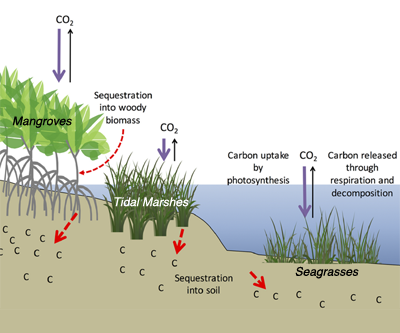
Comparatively, coastal wetlands (mangroves, tidal marshes, and seagrasses) effectively sequester carbon long-term (up to 10x more carbon stored per unit area than terrestrial forests with 50-90% of the stored carbon residing in the soil), and fall within clear national jurisdictions, which facilitates effective and quantifiable management actions. In addition, wetland degradation has the potential to release vast amounts of stored carbon back into the atmosphere and water column, meaning that conservation and restoration of these systems can also reduce potential emissions. The authors conclude that coastal wetland protection and restoration should be a primary focus in comprehensive climate change mitigation plans along with reducing emissions.

Authors:
Jennifer Howard (Conservation International)
Ariana Sutton-Grier (University of Maryland, NOAA)
Dorothée Herr (IUCN)
Joan Kleypas (NCAR)
Emily Landis (The Nature Conservancy)
Elizabeth Mcleod (The Nature Conservancy)
Emily Pidgeon (Conservation International)
Stefanie Simpson (Restore America’s Estuaries)

Original paper: http://onlinelibrary.wiley.com/doi/10.1002/fee.1451/full

Winter ventilation depth constrains the impact of the biological pump on CO2 uptake in the North Pacific Ocean

Posted by mmaheigan

· Thursday, June 8th, 2017

The North Pacific accounts for ~25% of the global ocean’s uptake of carbon dioxide (CO₂) from the atmosphere. However, the relative importance of the biological pump vs. physical circulation in driving ocean uptake of CO₂ remains poorly understood.

In a recent study, Palevsky and Quay (2017) used geochemical measurements collected on sixteen container ship transects between Hong Kong and Long Beach, CA to evaluate the drivers of CO₂ uptake across 8,000 kilometers in the North Pacific basin over the full annual cycle. In the eastern North Pacific, biologically-driven export of organic carbon below the winter ventilation depth fully offsets the uptake of CO₂ from the atmosphere. However, in the Kuroshio region of the western North Pacific, which has a deep winter mixed layer, the majority of the organic carbon exported during the productive summer season is subsequently respired and ventilated back to the atmosphere in winter. Subsequently, biologically-driven export offsets only a small fraction of the CO₂ uptake by the ocean and, instead, physical transport is the dominant process removing inorganic carbon from the region.

We further show that that mechanistic coupling between biological carbon export and ocean uptake of CO₂ from the atmosphere is sensitive to the seasonal timing of biological export and ventilation, as well as the magnitude of export. Future studies therefore need to measure biological carbon export and ventilation throughout the full annual cycle in order to better understand controls on regional variations in ocean CO₂ uptake rates and future changes in these rates.

Data from 16 shipboard transects across the North Pacific revealed a basin-wide gradient between the Kuroshio and Eastern regions in the relative roles of biological vs. physical processes in removing dissolved inorganic carbon from the surface ocean.

Authors:
Hilary I. Palevsky (Woods Hole Oceanographic Institution)
Paul D. Quay (University of Washington)

Do rivers supply nutrients to the open ocean?

Posted by mmaheigan

· Wednesday, May 24th, 2017

Rivers carry large amounts of nutrients (e.g., nitrogen and phosphorus) to the sea, but we do not know how much of that riverine nutrient supply escapes biological and chemical processing in shallow coastal waters to reach the open ocean. Most global ocean biogeochemical models, which are typically unable to resolve coastal processes, assume that either all or none of the riverine nutrients entering coastal waters actually contribute to open ocean processes.

While we know a good deal about the dynamics of individual rivers entering the coastal ocean, studies to date have been limited to a few major river systems, mainly in in developed countries. Globally, there are over 6,000 rivers entering the coastal ocean. In a recent study, Sharples et al (2017) devised a simple approach to obtain a global-scale estimate of riverine nutrient inputs based on the knowledge that low-salinity waters entering the coastal ocean tend to form buoyant plumes that turn under the influence of Earth’s daily rotation to flow along the coastline. Using published data on such flows and incorporating the effect of Earth’s rotation, they obtained estimates of typical cross-shore plume width and compared them to the local width of the continental shelf. This was used to calculate the residence time of riverine nutrients on the shelf, which is the key to estimating how much of a given nutrient is consumed in shelf waters vs. how much is exported to the open ocean.

Global distribution of the amount of riverine dissolved inorganic nitrogen that escapes the continental shelf to reach the open ocean.

The results indicate that, on a global scale, 75% (80%) of the nitrogen (phosphorus) supplied by rivers reaches the open ocean, whereas 25% (20%) of the nitrogen (phosphorus) is consumed on the shelf (e.g., fueling coastal productivity). Limited knowledge of nutrient cycling and consumption in shelf waters represents the primary source of uncertainty in this study. However, well-defined global patterns related to human land use (e.g., agricultural fertilizer use in developed nations) emerged from this analysis, underscoring the need to understand how land-use changes and other human activities will alter nutrient delivery to the coastal ocean in the future.

Authors:
Jonathan Sharples (School of Environmental Sciences, University of Liverpool, UK)
Jack Middelburg (Department of Earth Sciences, Utrecht University, Netherlands)
Katja Fennel (Department of Oceanography, Dalhousie University, Canada)
Tim Jickells (School of Environmental Sciences, University of East Anglia, UK)

Scientists reveal major drivers of aragonite saturation state in the Gulf of Maine, a region vulnerable to acidification

Posted by mmaheigan

· Thursday, May 11th, 2017

The Gulf of Maine (GoME) is a shelf region that is especially vulnerable to ocean acidification (OA). GoME’s shelf waters display the lowest mean pH, aragonite saturation state (Ω-Ar), and buffering capacity of the entire U.S. East Coast. These conditions are a product of many unique characteristics and processes occurring in the GoME, including relatively low water temperatures that result in higher CO₂ solubility; inputs of fresher, low-alkalinity water that is traceable to the rivers discharging into the Labrador Sea to the north, as well as local inputs of low-pH river water; and its semi-enclosed nature (long residence time >1 year), which enables the accumulation of respiratory products, i.e. CO₂.

A recent study by Wang et al. (2017) is the first to assess the major oceanic processes controlling seasonal variability of aragonite saturation state and its linkages with pteropod abundance in the GoME. The results indicate that surface production was tightly coupled with remineralization in the benthic nepheloid layer during highly productive seasons, resulting in occasional aragonite undersaturation. Mean water column Ω-Ar and abundance of large thecosomatous pteropods show some correlation, although discrete cohort reproductive success likely also influences their abundance. Photosynthesis-respiration is the primary driving force controlling Ω-Ar variability over the seasonal cycle. However, calcium carbonate (CaCO₃) dissolution appears to occur at depth in fall and winter months when bottom water Ω-Ar is generally low but slightly above 1. This is accompanied by a decrease in pteropod abundance that is consistent with previous CaCO₃ flux trap measurements.

Figure. Changes of aragonite saturation states (ΔΩ) between three consecutive cruises from April – July 2015 as a function of changes in salinity-normalized DIC (ΔenDIC, including correction of freshwater inputs) (a) and changes in salinity-normalized TA (ΔenTA, including correction of freshwater inputs) (b). The data points circled in (b) represent potential alkalinity sources from CaCO3 dissolution and/or anaerobic respiration. Solid lines are theoretical lines of ΔΩ vs. ΔenDIC and ΔΩ vs. ΔenTA expected if only photosynthesis and respiration/remineralization occur. Dashed lines are theoretical lines if only calcification and dissolution of CaCO3 occur.

Under the current rate of OA, the mean Ω-Ar of the subsurface and bottom waters of the GoME will approach undersaturation (Ω-Ar < 1) in 30-40 years. As photosynthesis and respiration are the major driving mechanisms of Ω-Ar variability in the water column, any biological regime changes may significantly impact carbonate chemistry and the GoME ecosystem, including the CaCO₃ shell-building capacity of organisms that are critical to the GoME food web.

Author:

Zhaohui Aleck Wang (Woods Hole Oceanographic Institution)

Biophysical drivers of vigorous carbon cycling near the Kuroshio Extension

Posted by mmaheigan

· Thursday, April 27th, 2017

The Kuroshio Current and its Extension jet in the western North Pacific Ocean form a dynamic western boundary current (WBC) region characterized by large air-sea exchanges of heat and carbon dioxide gas (CO₂). The jet is known to oscillate between stable and meandering states on multi-year timescales that alter the eddy field and depth of winter mixing in the southern recirculation gyre. These dynamic state changes have been shown to imprint biogeochemical signatures onto regional mode waters that can be distributed widely throughout the North Pacific and remain out of contact with the atmosphere for decades.

Figure. ~7 years of (a) AVISO daily sea surface height (SSH) anomalies and (b) upper-ocean temperature from the NOAA Kuroshio Extension Observatory (KEO) surface mooring. Black and gray lines in b show the mixed layer depth (MLD) and 17C contour, respectively. Spring bloom periods are indicated in blue in a. The semi-regular upwelling of cold water and corresponding depression of SSH is caused by cold-core eddies that pass the KEO mooring. Winter ventilation depths increase by ~100 m after 2010 when the extension jet entered a stable phase.

To better characterize carbon cycling in this region, ~7 years of daily-averaged autonomous CO₂ observations from NOAA’s Kuroshio Extension Observatory (KEO) surface mooring were used to close the mixed layer carbon budget. High rates of net community production (NCP; >100 mmol C m^-2 d^-1) were observed during the spring bloom period, and a mean annual NCP of 7±3 mol C m^-2 yr^-1 was determined. Biological processes near KEO largely balance the input of carbon that occurs annually through winter mixing; however, physical processes that deviate from climatology were not resolved in this study. Therefore, it remains unclear how transient features such as eddies influence biological carbon production and export through altered nutrient supply and active vertical transport of organic material. Further work is required to determine how biophysical interactions during mesoscale and submesoscale disturbances contribute to local carbon cycle processes and variability in regional mode water carbon inventories.

Ocean Carbon Hot Spots, an upcoming workshop focused on understanding biophysical drivers of carbon uptake in WBC regions, will be held September 25-26, 2017 at the Monterey Bay Aquarium Research Institute (MBARI) in Moss Landing, California. The primary objective of the workshop is to develop a community of observationalists and modelers working on the topic, and to identify critical observational needs that would improve model parameterizations. Ocean Carbon Hot Spots will be co-sponsored by US CLIVAR, US OCB, MBARI, and OMIX.

Written by Andrea J. Fassbender, Monterey Bay Aquarium Research Institute

Mixed-layer carbon cycling at the Kuroshio Extension Observatory (Global Biogeochemical Cycles)

Authors:
Andrea J. Fassbender (Monterey Bay Aquarium Research Institute)
Christopher L. Sabine (NOAA Paciﬁc Marine Environmental Laboratory)
Meghan F. Cronin (NOAA Paciﬁc Marine Environmental Laboratory)
Adrienne J. Sutton (Joint Institute for the Study of the Atmosphere and Ocean, University of Washington)

Satellite Laser Lights Up Polar Research

Posted by mmaheigan

· Thursday, April 13th, 2017

What controls annual cycles and interannual changes in polar phytoplankton biomass? Answers to this question are now emerging from a satellite light detection and ranging (lidar) sensor, which can observe the polar oceans throughout the extensive periods when measurements from traditional passive ocean color sensors are impossible. The new study uses active lidar measurements from the CALIOP satellite sensor to construct complete decade-long record of phytoplankton biomass in the northern and southern polar regions. Results of the study show that annual cycles in biomass are driven by rates of acceleration and deceleration in phytoplankton division, with bloom termination coinciding with maximum division rates irrespective of whether nutrients are exhausted. The study further shows that interannual differences in bloom strength can be quantitatively related to the difference between the winter minimum to summer maximum in division rates. Finally, the analysis indicated that ecological processes had a greater impact than ice cover changes on integrated polar zone phytoplankton biomass in the north, whereas ice cover changes were the dominant driver in the south polar zone. Despite being designed for atmospheric research, CALIOP has provided the first demonstration that active satellite lidar measurements can yield important new insights on plankton ecology in the climate sensitive polar regions. This proof-of-concept creates a foundation for a future ocean-optimized sensor with water-column profiling capabilities that would launch a new lidar era in satellite oceanography.

Authors:

Michael J. Behrenfeld (Oregon State Univ.)
Yongxiang Hu (NASA Langley Research Center)
Robert T. O’Malley (Oregon State Univ.)
Emmanuel S. Boss (Univ. Maine)
Chris A. Hostetler (NASA Langley Research Center)
David A. Siegel (Univ. California Santa Barbara)
Jorge Sarmiento (Princeton Univ.)
Jennifer Schulien (Oregon State Univ.)
Johnathan W. Hair (NASA Langley Research Center)
Xiaomei Lu (NASA Langley Research Center)
Sharon Rodier (NASA Langley Research Center)
Amy Jo Scarino (NASA Langley Research Center)

International team of researchers reports ocean acidification is spreading rapidly in the western Arctic Ocean

Posted by mmaheigan

· Thursday, March 30th, 2017

The Arctic Ocean is particularly sensitive to climate change and ocean acidification such that aragonite saturation state is expected to become undersaturated (Ω_arag <1) there sooner than in other oceans. However, the extent and expansion rate of ocean acidification (OA) in this region are still unknown.

In the March 2017 issue of Nature Climate Change, Qi et al. show that, between 1994 and 2010, low Ω_arag waters have expanded northwards at least 5º, to 85ºN, and deepened from 100 m to 250 m depth. Data from multiple trans-western Arctic Ocean cruises show that Ω_arag<1 water has increased in the upper 250 m from 5 to 31% of the total area north of 70ºN. Tracer data and model simulations suggest that increased transport of Pacific Winter Water (which is already acidified due to both natural and anthropogenic sources), driven by sea-ice retreat and the circulation changes, are primarily responsible for the expansion, while local carbon recycling and anthropogenic CO₂ uptake have also contributed. These results indicate more rapid acidification is occurring in the Arctic Ocean, two to four times faster than the Pacific and Atlantic Oceans, with the western Arctic Ocean the first open-ocean region with large-scale expansion of “acidified” water directly observed in the upper water column.

The rapid spread of ocean acidification in the western Arctic has implications for marine life, particularly clams, mussels and pteropods that may have difficulty building or maintaining their shells in increasingly acidified waters. The pteropods are part of the Arctic food web and important to the diet of salmon and herring. Their decline could affect the larger marine ecosystem.

Authors:
Richard A. Feely (NOAA Pacific Marine Environmental Laboratory)
Leif G. Anderson (Univ. of Gothenburg)
Heng Sun (SOA Third Institute of Oceanography)
Jianfang Chen (SOA Second Institute of Oceanography
Min Chen (Univ. of Delaware)
Liyang Zhan (SOA Third Institute of Oceanography)
Yuanhui Zhang (SOA Third Institute of Oceanography)
Wei-Jun Cai (Univ. of Delaware, Univ. of Georgia)

Funding for the Ocean Carbon & Biogeochemistry Project Office is provided by the National Science Foundation (NSF) and the National Aeronautics and Space Administration (NASA). The OCB Project Office is housed at the Woods Hole Oceanographic Institution.

Archive for New OCB Research – Page 26

FilterbyKeyword