Diel Vertically Migrating Zooplankton that spend their day in an Oxygen Deficient Zone to avoid predators are a previously ignored source of organic matter for N2 producing bacteria.
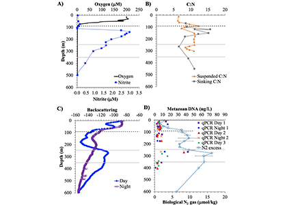
A recent study in GBC, examined biogeochemical cycling in the offshore Eastern Tropical North Pacific Oxygen Deficient Zone. They found that the daytime maximum in backscattering, used as a proxy for zooplankton and forage fish, corresponded to quantitative PCR maxima in zooplankton and forage fish (metazoan) DNA and to the maximum in biological N2 gas, and a shoulder of the nitrite maximum. At the same time, the C:N ratio of both suspended and sinking organic matter were reduced, indicating less degraded organic matter. These data strongly suggest that N2 production in the core of the Oxygen Deficient Zone is stimulated by the daily migration of zooplankton and forage fish in the Oxygen Deficient Zone. These results decouple N2 production from sinking organic matter fluxes. This work indicates that multicellular animals can affect key ocean biogeochemical cycles, and can cause hot spots of microbial activity well below the sunlit ocean.
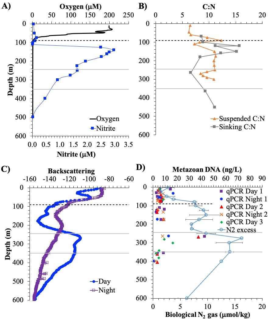
Figure caption: Offshore Eastern Tropical North Pacific Oxygen Deficient Zone. The dashed black line indicates the top of the ODZ, the gray lines indicate the boundaries of the deep vertical migration maximum. A) Concentrations of nitrite and oxygen, B) C:N of suspended and of sinking (sediment trap) organic matter, C) Day and night backscattering, a proxy for zooplankton and forage fish, and D) Biological N2 gas concentrations and day and night quantitative PCR data for zooplankton and forage fish (metazoans).
Authors
Clara Fuchsman (UMCES Horn Point Laboratory)
Megan Duffy (Univ Vermont)
Jacob Cram (UMCES Horn Point Laboratory)
Paulina Huanca-Valenzuela (UMCES Horn Point Laboratory)
Louis Plough (UMCES Horn Point Laboratory)
James Pierson (UMCES Horn Point Laboratory)
Catherine Fitzgerald (UMCES Horn Point Laboratory)
Allan Devol (U. of Washington)
Richard Keil (U. of Washington)
Paper: https://agupubs.onlinelibrary.wiley.com/doi/full/10.1029/2024GB008365