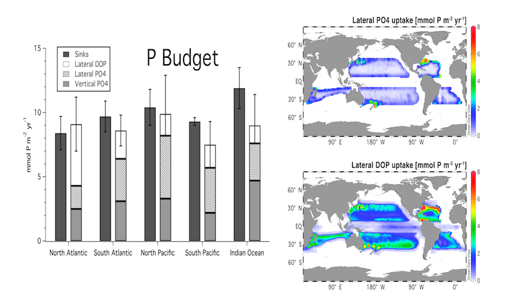
Vertical processes are thought to dominate nutrient resupply across the ocean, however estimated vertical fluxes are insufficient to sustain observed net productivity in the thermally stratified subtropical gyres. A recent study by Letscher et al. (2016) published in Nature Geoscience used a global biogeochemical ocean model to quantify the importance of lateral transport and biological uptake of inorganic and organic forms of nitrogen and phosphorus to the euphotic zone over the low-latitude ocean. Lateral nutrient transport is a major contributor to subtropical nutrient budgets, supplying a third of the nitrogen and up to two-thirds of the phosphorus needed to sustain gyre productivity. Half of the annual lateral nutrient flux occurs during the stratified summer and fall months, helping to explain seasonal patterns of net community production at the time-series sites near Bermuda and Hawaii. Figure from Letscher et al. (2016).