Blue carbon ecosystems—mangroves, saltmarshes, and seagrass meadows—carbon sequestration powerhouses that can help us mitigate climate change. For many years, our community has focused on studying and quantifying organic carbon storage in the soils of these ecosystems and crediting it as Blue Carbon in carbon markets.
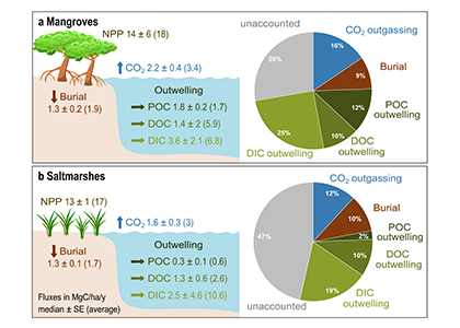
A new paper in Nature Communications reveals that much of that carbon sequestered by mangroves and saltmarshes is actually exported as inorganic carbon to the ocean. Inorganic carbon export dominates blue carbon budgets and rivals or even surpasses carbon stored in soils. Inorganic carbon exports had an alkalinity: dissolved inorganic carbon ratio of 0.8 ± 0.2, impacting the carbonate system and carbon cycling along the coast. Most of the inorganic carbon is exported as bicarbonate which stays permanently dissolved in the ocean and is therefore a permanent atmospheric carbon sink. When we ignore inorganic carbon export, we highly underestimate the potential of mangroves and saltmarshes to mitigate climate change. Consequently, inorganic carbon export should be integrated into blue carbon frameworks to adequately inform carbon markets, which encourage landowners to restore and preserve mangrove and saltmarsh ecosystems.

Authors
Gloria M. S. Reithmaier (University of Gothenburg) Twitter: @GReithmaier@Barefoot_Lab
Alex Cabral (University of Gothenburg)
Anirban Akhand (Hong Kong University of Science and Technology)
Matthew J. Bogard (University of Lethbridge)
Alberto V. Borges (University of Liège)
Steven Bouillon (KU Leuven)
David J. Burdige (Old Dominion University)
Mitchel Call (Southern Cross University)
Nengwang Chen (Xiamen University)
Xiaogang Chen (Westlake University)
Luiz C. Cotovicz Jr (Leibniz Institute for Baltic Sea Research)
Meagan J. Eagle (U.S. Geological Survey)
Erik Kristensen (University of Southern Denmark)
Kevin D. Kroeger (U.S. Geological Survey)
Zeyang Lu (Xiamen University)
Damien T. Maher (Southern Cross University)
Lucas J. Pérez-Lloréns (University of Cádiz)
Raghab Ray (University of Tokyo)
Pierre Taillardat (National University of Singapore)
Joseph J. Tamborski (Old Dominion University)
Rob C. Upstill-Goddard (Newcastle University)
Faming Wang (Chinese Academy of Sciences)
Zhaohui Aleck Wang (Woods Hole Oceanographic Institution)
Kai Xiao (Southern University of Science and Technology)
Yvonne Y. Y. Yau (University of Gothenburg)
Isaac R. Santos (University of Gothenburg)