On the evening of February 19, 2024 members of the Gulf of Mexico (GMx) Regional Node Working Group on Marine Carbon Dioxide Removal (mCDR) met for the first time. They kicked off the first night of the Ocean Sciences Meeting in New Orleans, a week for oceanographers across all disciplines to share their work. The evening began with a networking hour co-hosted by Carbon to Sea, Exploring Ocean Iron Solutions (ExOIS), [C]Worthy, and Ocean Visions. Leaders from the mCDR industry gathered amid the bluish glow of the tarpon exhibit at the Audubon Aquarium for a night of meaningful conversation and shared connections. After networking, members of the GMx node group moved to a breakout room for their own meeting.
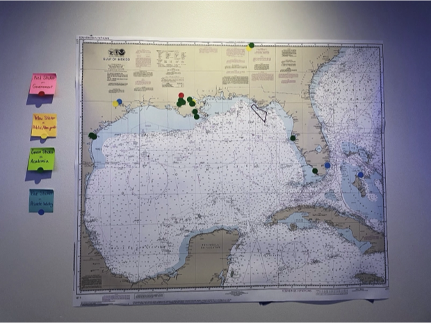
This launched a new effort to address climate challenges in the Gulf Coast's unique ecological landscape. Framed by its vital connection to the Caribbean Sea through the dynamic Gulf Stream, GMx is nourished and challenged by the substantial discharge from the Mississippi River. This area is a nexus of environmental contrasts, grappling with coastal hazards such as hurricanes, escalating sea level rise, and the distressing phenomenon of coral reef bleaching.
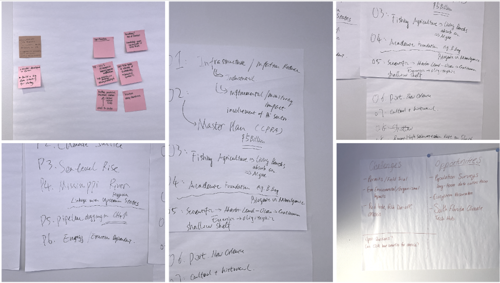
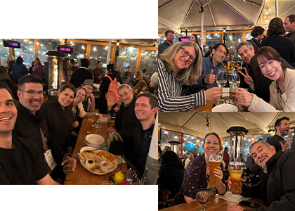
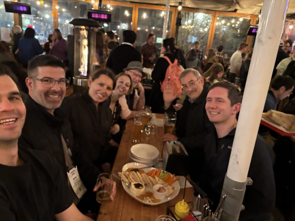
Marine carbon dioxide removal has the potential to shape the future of the Gulf. Members sharing this belief attended the meeting to connect through local knowledge and goal setting. Nineteen participants from the Gulf region and beyond, including Louisiana, Texas, Florida, Georgia, and the Bahamas, participated in a series of interactive activities (Figure 1). After introductions, they clustered into groups according to these regions of origin and were asked to highlight several challenges and opportunities unique to their area. A few of these opportunities are:
- High nutrient and carbon input from the Mississippi River, enhancing primary productivity.
- The river’s buoyancy extends the residence time of coastal waters, facilitating sediment settling and potentially enhancing mCDR.
- Integrating wetlands, estuarine, and marine environments supports diverse mCDR strategies.
- Existing oil and gas infrastructure could support new mCDR initiatives, with significant interest from the private sector.
These challenges and opportunities then became the center of discussion. While consensus on specific actions was not reached, the group found a common interest in the environmental and socio-economic impacts of mCDR. Members closed the session by sharing two personal or professional goals for the upcoming year.
Moving forward, the group strategy involves seeking co-production opportunities with industry and non-profit partners. Possible projects include the development of an MRV (Monitoring, Reporting, and Verification) toolbox and a foundational study outlining regional mCDR opportunities. Highlighting these opportunities is essential to attract government and private investment and unite stakeholders around shared objectives. The newly formed GMx node left their kickoff meeting feeling energized to develop these plans further and launch them into action.
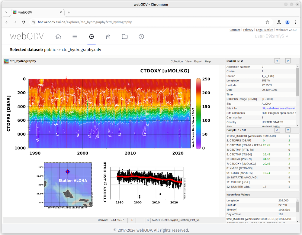 One of the longest running open ocean time-series on our planet, the Hawaii Ocean Time-series (HOT) can now be accessed using webODV at