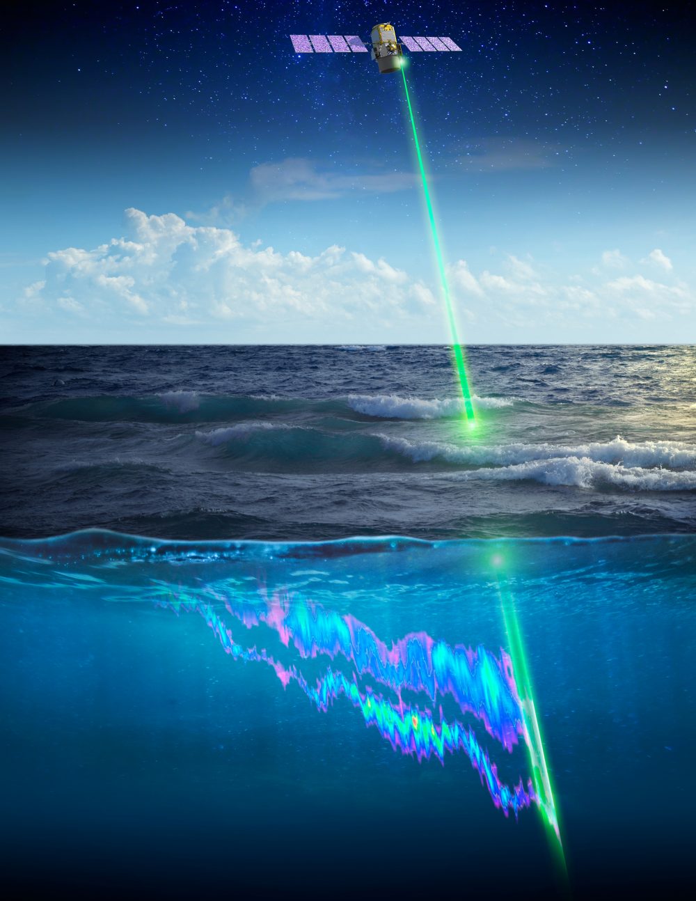
Ocean Carbon & Biogeochemistry
Studying marine ecosystems and biogeochemical cycles in the face of environmental change
  • Home
  • About OCB
    • About Us
    • Scientific Breadth
      • Biological Pump
      • Changing Marine Ecosystems
      • Changing Ocean Chemistry
      • Estuarine and Coastal Carbon Fluxes
      • Ocean Carbon Uptake and Storage
      • Ocean Observatories
    • Code of Conduct
    • Get Involved
    • Project Office
    • Scientific Steering Committee
    • OCB committees
      • Ocean Time-series
      • US Biogeochemical-Argo
      • Ocean-Atmosphere Interaction
  • Activities
    • Summer Workshop
    • OCB Webinars
    • Guidelines for OCB Workshops & Activities
    • Topical Workshops
      • CMIP6 Models Workshop
      • Coastal BGS Obs with Fisheries
      • C-saw extreme events workshop
      • Expansion of BGC-Argo and Profiling Floats
      • Fish, fisheries and carbon
      • Future BioGeoSCAPES program
      • GO-BCG Scoping Workshop
      • Lateral Carbon Flux in Tidal Wetlands
      • Leaky Deltas Workshop – Spring 2025
      • Marine CDR Workshop
      • Ocean Nucleic Acids ‘Omics
      • Pathways Connecting Climate Changes to the Deep Ocean
    • Small Group Activities
      • Aquatic Continuum OCB-NACP Focus Group
      • Arctic-COLORS Data Synthesis
      • BECS Benthic Ecosystem and Carbon Synthesis WG
      • Carbon Isotopes in the Ocean Workshop
      • CMIP6 WG
      • Filling the gaps air–sea carbon fluxes WG
      • Fish Carbon WG
      • Meta-eukomics WG
      • mCDR
      • Metaproteomic Intercomparison
      • Mixotrophs & Mixotrophy WG
      • N-Fixation WG
      • Ocean Carbonate System Intercomparison Forum
      • Ocean Carbon Uptake WG
      • OOI BGC sensor WG
      • Operational Phytoplankton Observations WG
      • Phytoplankton Taxonomy WG
    • Other Workshops
    • Science Planning
      • Coastal CARbon Synthesis (CCARS)
      • North Atlantic-Arctic
    • Ocean Acidification PI Meetings
    • Training Activities
      • PACE Hackweek 2025
      • PACE Hackweek 2024
      • PACE Training Activity 2022
  • Science Support
    • Data management and archival
    • Early Career
    • Funding Sources
    • Jobs & Postdocs
    • Meeting List
    • OCB Topical Websites
      • Ocean Fertilization
      • Trace gases
      • US IIOE-2
    • Outreach & Education
    • Promoting your science
    • Student Opportunities
    • OCB Activity Proposal Solicitations
      • Guidelines for OCB Workshops & Activities
    • Travel Support
  • Publications
    • OCB Workshop Reports
    • Science Planning and Policy
    • Newsletter Archive
  • Science Highlights
  • News

Archive for phytoplankton – Page 6

Oceanic fronts enhance carbon transport to the ocean’s interior through both subduction and amplified sinking

Posted by mmaheigan 
· Wednesday, March 1st, 2017 

Mesoscale fronts are regions with potentially enhanced nutrient fluxes, phytoplankton production and biomass, and aggregation of mesozooplankton and higher trophic levels. However, the role of these features in transporting organic carbon to depth and hence sequestering CO2 from the atmosphere has not previously been determined. Working with the California Current Ecosystem Long Term Ecological Research (CCE LTER) program, we determined that the flux of sinking particles at a stable front off the coast of California was twice as high as similar fluxes on either side of the front, or in typical non-frontal waters of the CCE in a recent study by Stukel et al. (2017) published in Proceedings of the National Academy of Sciences.

This increased export flux was tied to enhanced silica-ballasting by Fe-stressed diatoms and to an abundance of mesozooplankton grazers. Furthermore, downward transport of particulate organic carbon by subduction at the front led to additional carbon export that was similar in magnitude to sinking flux, suggesting that these fronts (which are a common feature in productive eastern boundary upwelling systems) are an important conduit for carbon sequestration. These enhanced carbon export mechanisms at episodic and mesoscale features need to be included in future biogeochemical forecast models to understand how a changing climate will affect marine CO2 uptake.

Authors

Michael R. Stukel (Florida State University)
Lihini I. Aluwihare, Katherine A. Barbeau, Ralf Goericke, Arthur J. Miller, Mark D. Ohman, Angel Ruacho, Brandon M. Stephens, Michael R. Landry (University of California, San Diego)
Hajoon Song (Massachusetts Institute of Technology)
Alexander M. Chekalyuk (Lamont-Doherty Earth Observatory)

ENSO impacts on ecosystem indicators in the California Current System

Posted by mmaheigan 
· Thursday, February 16th, 2017 

El Niño-Southern Oscillation (ENSO) events activate long-distance teleconnections through the atmosphere and ocean that can dramatically impact marine ecosystems along the West Coast of North America, affecting diverse organisms ranging from plankton to exploitable and protected species. Such ENSO-related changes to marine ecosystems can ultimately affect humans in many ways, including via depressed plankton and fish production, dramatic range shifts for many protected and exploited species, inaccessibility of traditionally fished resources, more prevalent harmful algal blooms, altered oxygen and pH of waters used in mariculture, and proliferation of pathogens. The principal objective of the Forecasting ENSO Impacts on Marine Ecosystems of the US West Coast workshop was to develop a scientific framework for building an ENSO-related forecast system of ecosystem indicators along the West Coast of North America, including major biological and biogeochemical responses. Attendees realized that a quantitative, biologically-focused forecast system is a much more challenging objective than forecasting the physical system alone; it requires an understanding of the ocean-atmospheric physical system and of diverse organism-level, population-level, and geochemical responses that, in aggregate, lead to altered ecosystem states.

In the tropical ocean, important advances have been made in developing both intensive observational infrastructure (Global Tropical Moored Buoy Array) and diverse dynamical and statistical models that utilize these data in ENSO forecasting. These forecasts are made widely available (e.g., NOAA’s Climate Prediction Center). The most sophisticated ENSO-forecasting efforts use global, coupled ocean-atmosphere climate models that extend ENSO-forecasting skill into seasonal climate forecasting skill for other regions, including the California Current System (CCS). However, both these measurement systems and forecast models are restricted to the physical dynamics of ENSO, rather than biotic and biogeochemical consequences.

Primary modes of influence of El Niño on marine organisms

In this brief discussion, we focus primarily on the warm (El Niño) phases of ENSO, which can have large and generally negative ecosystem consequences, although changes accompanying the cold phases (La Niña) can also be significant. We primarily address pelagic ocean processes, which merely reflect the expertise of the participants at the workshop. Physical mechanisms by which ENSO impacts the U.S. West Coast are more completely explained in Jacox et al. (this issue).

El Niño affects organisms and biogeochemistry via both local and advective processes (Figure 1). ENSO-related changes in the tropics can affect the CCS through an atmospheric teleconnection (Alexander et al. 2002) to alter local winds and surface heat fluxes, and through upper ocean processes (thermocline and sea level displacements and geostrophic currents) forced remotely by poleward propagating coastally trapped waves (CTWs) of tropical origin (Enfield and Allen 1980; Frischkencht et al. 2015; Figure 1). It is important to recognize that ecosystem effects will occur through three primary mechanisms: (1) via the direct action of altered properties like temperature, dissolved O2, and pH on the physiology and growth of marine organisms; (2) through food web effects as changes in successive trophic levels affect their predators (bottom up) or prey (top down); and (3) through changes in advection related to the combination of locally forced Ekman transport and remotely forced geostrophic currents, typically involving poleward and/or onshore transport of organisms. Advective effects can be pronounced, transporting exotic organisms into new regions and altering the food web if these imported species have significant impacts as predators, prey, competitors, parasites, or pathogens.

Figure 1. Schematic illustration of dominant mechanisms through which ENSO impacts biological and biogeochemical processes in the California Current System. Processes include both local effects (e.g., heat budget, winds) and advective effects. Such processes can influence organisms via: (1) (yellow arrow) direct physiological responses to changes in temperature, O2, pH, etc.; (2) (orange arrows) effects that propagate through the food web, as successive trophic levels affect their predators (bottom up, upward-facing orange arrows) or prey (top down, downward-facing orange arrows); (3) (blue arrows) direct transport effects of advection. Top predators are not included here. CTW indicates coastally trapped waves.


I. Poleward and onshore transport

Active, mobile marine fishes, seabirds, reptiles, and mammals may move into new (or away from old) habitats in the CCS as ENSO-related changes occur in the water column and render the physical-chemical characteristics and prey fields more (or less) suitable for them. Planktonic organisms are often critical prey and are, by definition, subject to geographic displacements as a consequence of altered ocean circulation that accompanies El Niño events. Most commonly, lower latitude organisms are transported poleward to higher latitudes in either surface flows or in an intensified California Undercurrent (Lynn and Bograd 2002). However, some El Niño events are accompanied by onshore flows (Simpson 1984), potentially displacing offshore organisms toward shore (Keister et al. 2005).

Two of the most celebrated examples of poleward transport come from distributions of pelagic red crabs (Pleuroncodes planipes) and the subtropical euphausiid (or krill, Nyctiphanes simplex), both of which have their primary breeding populations in waters off Baja California, Mexico (Boyd 1967; Brinton et al. 1999). Pelagic red crabs were displaced approximately 10° of latitude, from near Bahia Magdalena, Baja California, northward to Monterey, California (Glynn 1961; Longhurst 1967) during the El Niño of 1958-1959. This early event was particularly well documented because of the broad latitudinal coverage of the California Cooperative Oceanic Fisheries Investigations (CalCOFI) cruises at the time. Such El Niño-related northward displacements have been documented repeatedly over the past six decades (McClatchie et al. 2016), partly because the red crabs often strand in large windrows on beaches and are conspicuous to the general public. The normal range of the euphausiid Nyctiphanes simplex is centered at 25-30°N (Brinton et al. 1999). N. simplex has been repeatedly detected far to the north of this range during El Niño, extending at least to Cape Mendocino (40.4°N) in 1958 (Brinton 1960), to northern Oregon (46.0°N) in 1983 (Brodeur 1986), and to Newport, Oregon (44.6°N; Keister et al. 2005) and northwest Vancouver Island (50.7°N; Mackas and Galbraith 2002) in 1998. In spring of 2016, N. simplex were extremely abundant in the southern California region (M. Ohman and L. Sala, personal communication) and detected as far north as Trinidad Head (41.0°N) but not in Newport, Oregon (W. Peterson, personal communication). Sometimes such El Niño-related occurrences of subtropical species are accompanied by declines in more boreal species (e.g., Mackas and Galbraith 2002; Peterson et al. 2002), although this is not always the case.

Among the organisms displaced during El Niños, the consequences of transport of predators are poorly understood but likely significant in altering the food web.  Subtropical fishes can be anomalously abundant in higher latitudes during El Niño (Hubbs 1948; Lluch-Belda et al. 2005; Pearcy and Schoener 1987; Pearcy 2002; Brodeur et al. 2006), with significant consequences for the resident food web via selective predation on prey populations.

II. Habitat compression

Many species are confined to a specific habitat that may compress during El Niño. This phenomenon has been observed repeatedly for species and processes related to coastal upwelling in the CCS. During major El Niño events, as the offshore extent of upwelled waters is reduced and becomes confined close to the coast, the zone of elevated phytoplankton (observed as Chl-a) compresses markedly to a narrow zone along the coastal boundary (e.g., Kahru and Mitchell 2000; Chavez et al. 2002). For example, during the strong El Niño spring of 1983, the temperate euphausiid Euphausia pacifica was present in low densities throughout Central and Southern California waters, but 99% of the biomass was unusually concentrated at a single location (station 80.51) very close to Point Conception, where upwelling was still pronounced (E. Brinton, personal communication). The spawning habitat of the Pacific sardine (Sardinops sagax) was narrowly restricted to the coastal boundary during El Niño 1998, but one year later during La Niña 1999, the spawning habitat extended a few hundred kilometers farther offshore (Lo et al. 2005). Market squid, Doryteuthis opalescens, show dramatically lower catches during El Niño years (Reiss et al. 2004), but in 1998, most of the catch was confined to a small region in Central California (Reiss et al. 2004). During the El Niño in spring 2016, vertical particle fluxes measured by sediment traps were reduced far offshore but remained elevated in the narrow zone of coastal upwelling very close to Point Conception (M. Stukel, personal communication).

III. Altered winds and coastal upwelling

Upwelling-favorable winds along the US West Coast may decline during El Niño conditions (Hayward 2000, but see Chavez et al. 2002) and vertical transports can be reduced (Jacox et al. 2015), mainly during the winter and early spring (Black et al. 2011). Independent of any changes in density stratification (considered below), these decreased vertical velocities can lead to diminished nutrient fluxes, reduced rates of primary production, and a shift in the size composition of the plankton community to smaller phytoplankton and zooplankton (Rykaczewski and Checkley 2008). Such changes at the base of the food web can have major consequences for a sequence of consumers at higher trophic levels, as both the concentration and suitability of prey decline.

However, there are potential compensatory effects of reduced rates of upwelling. Diminished upwelling also means less introduction of CO2-rich, low-oxygen waters to coastal areas (Feely et al. 2008; Bednaršek et al. 2014), with potential benefits to organisms that are sensitive to calcium carbonate saturation state or hypoxic conditions. Furthermore, reduced upwelling implies lower Ekman transport and potentially reduced cross-shore fluxes far offshore within coastal jets and filaments (cf., Keister al. 2009).

IV. Increased stratification and deepening of nutricline

El Niño-related warming of surface waters and increased density stratification can result from advection of warmer waters and/or altered local heating. Evidence suggests that the pycnocline (Jacox et al. 2015) and nitracline (Chavez et al. 2002) deepen during stronger El Niños. This effect, independent of variations in wind stress, also leads to diminished vertical fluxes of nitrate and other limiting nutrients and suppressed rates of primary production. Decreased nitrate fluxes appear to explain elevated 15N in California Current zooplankton (Ohman et al. 2012) and decreased krill abundance (Lavaniegos and Ohman 2007; Garcia-Reyes et al. 2014) during El Niño years. For example, the 2015-16 El Niño resulted in a pronounced warming of surface waters and depressed Chl-a concentrations across a broad region of the CCS (McClatchie et al. 2016).

V. Direct physiological responses to altered temperature, dissolved O2, pH

Most organisms in the ocean—apart from some marine vertebrates—are ectothermic, meaning they have no capability to regulate their internal body temperature. Heating or cooling of the ocean therefore directly influences their rates of metabolism, growth, and mortality. Most organisms show not only high sensitivity to temperature variations but nonlinear responses. A typical temperature response curve or “thermal reaction norm” (e.g., of growth rate) is initially steeply positive with increasing temperature, followed by a narrow plateau, then abruptly declines with further increases in temperature (e.g., Eppley 1972). Different species often show different thermal reaction norms. Hence, El Niño-related temperature changes may not only alter the growth rates and abundances of organisms, but also shift the species composition of the community due to differential temperature sensitivities.

Similarly, El Niño-induced variations in dissolved oxygen concentration and pH can have marked consequences for physiological responses of planktonic and sessile benthic organisms and, for active organisms, potentially lead to migrations into or out of a suitable habitat. Interactions between variables (Boyd et al. 2010) will also lead to both winners and losers in response to major ENSO-related perturbations.

Altered parasite, predator populations, and harmful algal blooms

ENSO-related changes can favor the in situ proliferation or introduction of predators, parasites, pathogens, and harmful algal blooms. Such outbreaks can have major consequences for marine ecosystems, although some are relatively poorly studied. For example, a recent outbreak of sea star wasting disease thought to be caused by a densovirus adversely affected sea star populations at numerous locations along the West Coast (Hewson et al. 2014). While not specifically linked to El Niño, this outbreak was likely tied to warmer water temperatures. Because some sea stars are keystone predators capable of dramatically restructuring benthic communities (Paine 1966), such pathogen outbreaks are of considerable concern well beyond the sea stars themselves.

Domoic acid outbreaks, produced by some species of the diatom genus Pseudo-nitzschia, can result in closures of fisheries for razor clams, Dungeness crab, rock crab, mussels, and lobsters, resulting in significant economic losses. While the causal mechanisms leading to domoic outbreaks are under discussion (e.g., Sun et al. 2011; McCabe et al. 2016), warmer-than-normal ocean conditions in northern regions of the CCS have been linked to domoic acid accumulation in razor clams, especially when El Niño conditions coincide with the warm phase of the Pacific Decadal Oscillation (McKibben et al. 2017).

ENSO diversity, non-stationarity, and consequences of secular changes

There is considerable interest in understanding the underlying dynamical drivers that lead to different El Niño events (Singh et al. 2011; Capotondi et al. 2015). Although there appears to be a continuum of El Niño expression along the equatorial Pacific, some simplify this continuum to a dichotomy between Eastern Pacific (EP) and Central Pacific (CP) events (Capotondi et al 2015). Whether EP and CP El Niños have different consequences for mid-latitude ecosystems like the California Current Ecosystem is an area of open research, but some evidence suggests that differences in timing and intensity of biological effects may exist (cf. Fisher et al. 2015). While some studies (e.g., Lee and McPhaden 2010) suggest that the frequency of CP El Niños is increasing, the evidence is not definitive (Newman et al. 2011). In addition to questions about the ecosystem consequences of El Niño diversity, there are unknowns regarding interactions between El Niño, decadal-scale variability (Chavez et al. 2002), and secular changes in climate (Figure 2, Ohman, unpubl.), which suggest a non-stationary relationship between California Current zooplankton and El Niño. An index of the dominance of warm water krill from CalCOFI sampling in Southern California shows that for the first 50 years there was a predictable positive relationship between these warm water krill and El Niño. This relationship held during both EP and CP El Niño events from 1950-2000. However, the relationship appeared to weaken after 2000. The warm water krill index was negatively correlated with the moderate El Niño of 2009-10. While the krill index again responded to the major El Niño of 2015-16 and the preceding year of warm anomalies (Bond et al. 2015; Zaba and Rudnick 2016), the magnitude of the response was not comparable to what had been seen in earlier decades. It is unclear whether such results are merely the consequence of interannual variability in the mode of El Niño propagation (Todd et al. 2011) or a change in the relationship between El Niño forcing and ecosystem responses.


Figure 2. Covariability of California Current euphausiids (krill, blue lines) with an index of ENSO off California (de-trended sea level anomaly [DTSLA] at San Diego, green lines). Note the markedly different relationship between euphausiids and DTSLA after 2000. Sustained excursions of DTSLA exceeding one standard deviation (i.e., above upper dotted red line) are expressions of El Niño (or of the warm anomaly of 2014-2015). Red arrows indicate specific events categorized as either eastern Pacific (EP) or central Pacific (CP) El Niño events (Yu et al. 2012), apart from 2015-2016 which could be either CP or EP. The Warm-Cool euphausiid index is based on the difference in average log carbon biomass anomaly of the four dominant warm water euphausiids in the CCS minus the average anomaly of the four dominant cool water euphausiids (species affinities from Brinton and Townsend 2003). Euphausiid carbon biomass from springtime CalCOFI cruises off Southern California, lines 77-93, nighttime samples only. Dotted blue lines indicate years of no samples (Ohman, personal communication).

Conclusions

While the potential modes of El Niño influence on biological and biogeochemical processes in the CCS are numerous, not all processes are of first order consequence to all organisms. Forecasting ENSO effects on a given target species will likely focus on a limited number of governing processes. Table 1 illustrates some of the specific types of organisms susceptible to El Niño perturbations and the suspected dominant mechanism. We look forward to developing a framework for forecasting such responses in a quantitative manner.

Ecosystem indicator Region and season Change during El Niño Time scale of response Regional ocean processes
Primary production Entire CCS

winter, spring, summer

Declines Variable lag;

Instantaneous or time-lagged

Reduced upwelling, nutrient fluxes; Deeper nutricline and weaker winds
Pseudo-nitzschia diatoms; Domoic Acid Entire CCS

spring-summer

Blooms  

1-3 month lag

Elevated temperature; Altered nutrient stoichiometry
Copepod assemblage NCCS

spring-summer

Warm water species appear Nearly instantaneous Poleward advection; Reduced upwelling, warmer temperature
 

Subtropical euphausiids


SCCS

spring-summer


Increase

Nearly instantaneous; persists beyond Niño event Poleward advection
Cool water euphausiids Entire CCS

spring-summer

Decrease Time-lagged Reduced upwelling; Anomalous advection
Pelagic red crabs SCCS & CCCS

winter, spring, summer

Increase Nearly instantaneous Poleward advection
Market squid CCCS & SCCS

winter & spring

Collapse Instantaneous for distribution; time-lagged for recruitment Warmer temperature/deeper thermocline; Reduces spawning habitat
Pacific sardine Entire CCS

winter-spring

Changes in distribution;

Compression of spawning habitat

Instantaneous for spawning and distribution, recruitment time-lagged, biomass is time-integrated Wind stress, cross-shore transport


Northern anchovy CCCS & SCCS

winter-spring

Changes in distribution;

Compression of spawning habitat

Instantaneous for spawning and distribution, recruitment time-lagged, biomass is time-integrated Reduced upwelling; Anomalous advection


Juvenile salmon survival NCCS

spring-summer

Decrease in Pacific NW Time-integrated Reduce river flow, decreased food supply in ocean
Adult sockeye salmon

(Fraser River)

NCCS

summer

Return path deflected northward to Canadian waters Time-integrated Ocean temperature, including Ekman controls
Warm assemblage of mesopelagic fish SCCS

spring (?)

Increase Lagged 0-3 months Poleward and onshore advection
Common murre

(reproductive success)

CCCS

winter-spring

Decrease Time-Lagged, time-integrated Prey (fish) availability; Thermocline depth; Decreased upwelling?
Top predator reproduction and abundance Entire CCS Species-dependent Time-integrated Advection of prey, altered temperature, upwelling, mesoscale structure
Top predator distribution Entire CCS Altered geographic distributions Instantaneous or time-lagged Advection of prey, altered temperature, upwelling, mesoscale structure
Table 1.   Examples of water column biological processes and organisms known to be affected by El Niño in the California Current System. Columns indicate the type of organism; approximate geographic region and season of the effect; direction of change in response to El Niño; temporal pattern of response (immediate, time-lagged, time-integrated); and the hypothesized oceanographic processes driving the organism response. CCS = California Current System; NCCS, CCCS, and SCCS denote northern, central, and southern sectors of the CCS.


Authors

Mark D. Ohman (Scripps Institution of Oceanography)
Nate Mantua (NOAA Southwest Fisheries Science Center)
Julie Keister (University of Washington)
Marisol Garcia-Reyes (Farallon Institute)
Sam McClatchie (NOAA Southwest Fisheries Science Center)

References

Alexander, M. A., I. Blade, M. Newman, J. R. Lanzante, N. C. Lau, and J. D. Scott, 2002: The atmospheric bridge: The influence of ENSO teleconnections on air-sea interaction over the global oceans. Journal of Climate, 15, 2205-2231, doi: 10.1175/1520-0442(2002)015<2205:TABTIO>2.0.CO;2

Bednaršek, N., R. A. Feely, J. C. P. Reum, B. Peterson, J. Menkel, S. R. Alin, and B. Hales, 2014: Limacina helicina shell dissolution as an indicator of declining habitat suitability owing to ocean acidification in the California Current Ecosystem. Proc. Roy. Soc. B-Biolog. Sci., 281, doi: 10.1098/rspb.2014.0123.

Black, B. A., I. D. Schroeder, W. J. Sydeman, S. J. Bograd, B. K. Wells, and F. B. Schwing, 2011: Winter and summer upwelling modes and their biological importance in the California Current Ecosystem. Glob. Change Bio., 17, 2536-2545, doi: 10.1111/j.1365-2486.2011.02422.x.

Bond, N. A., M. F. Cronin, H. Freeland, and N. Mantua, 2015: Causes and impacts of the 2014 warm anomaly in the NE Pacific. Geophy. Res. Lett., 42, 3414-3420, doi: 10.1002/2015GL063306.

Boyd, C. M., 1967: The benthic and pelagic habitats of the red crab, Pleuroncodes planipes. Pacific Science, 21, 394-403.

Boyd, P. W., R. Strzepek, F. X. Fu, and D. A. Hutchins, 2010: Environmental control of open-ocean phytoplankton groups: Now and in the future. Limnol. Oceanogr., 55, 1353-1376, doi: 10.4319/lo.2010.55.3.1353.

Brinton, E., 1960: Changes in the distribution of euphausiid crustaceans in the region of the California Current. CalCOFI Reports, 7, 137-146, http://www.calcofi.org/publications/calcofireports/v07/Vol_07_Brinton.pdf.

Brinton, E., M. D. Ohman, A. W. Townsend, M. D. Knight, and A. L. Bridgeman, 1999: Euphausiids of the World Ocean. Vol. CD-ROM, MacIntosh version 1.0, UNESCO Publishing.

Brodeur, R. D., 1986: Northward displacement of the euphausiid Nyctiphanes simplex Hansen to Oregon and Washington waters following the El Niño event of 1982-83. J. Crustacean Bio., 6, 686-692, doi: 10.2307/1548382.

Brodeur, R. D., S. Ralston, R. L. Emmett, M. Trudel, T. D. Auth, and A. J. Phillips, 2006: Anomalous pelagic nekton abundance, distribution, and apparent recruitment in the northern California Current in 2004 and 2005. Geophy. Res. Lett., 33, doi:10.1029/2006gl026614.

Capotondi, A., and Coauthors, 2015: Understanding ENSO Diversity. Bull. Amer. Meteor. Soc., 96, 921-938, doi: 10.1175/BAMS-D-13-00117.1.

Chavez, F. P., and Coauthors, 2002: Biological and chemical consequences of the 1997–1998 El Niño in central California waters. Prog. Oceanogr., 54, 205-232, doi: 10.1016/S0079-6611(02)00050-2.

Enfield, D., and J. Allen, 1980: On the structure and dynamics of monthly mean sea-level anomalies along the Pacific coast of North and South America. J. Phys. Oceanogr., 10, 557–578, doi: 10.1175/1520-0485(1980)010<0557:OTSADO>2.0.CO;2.

Eppley, R. W., 1972: Temperature and phytoplankton growth in the sea. Fish. Bull, 70, 1063-1085, http://fishbull.noaa.gov/70-4/eppley.pdf.

Feely, R. A., C. L. Sabine, J. M. Hernandez-Ayon, and D. H. Ianson, B., 2008: Evidence for upwelling of corrosive “acidified” water onto the continental shelf. Science, 320, 1490-1492, doi: 10.1126/science.1155676.

Fisher J. L., W. T. Peterson, and R. R. Rykaczewski, 2015: The impact of El Niño events on the pelagic food chain in the northern California Current. Glob. Change Bio., 21, 4401–4414, doi: 10.1111/gcb.13054.

Frischknecht, M., M. Münnich, and N. Gruber, 2015: Remote versus local influence of ENSO on the California Current System, J. Geophys. Res. Oceans, 120, 1353–1374, doi:10.1002/2014JC010531.

García-Reyes, M., J. L. Largier, and W. J. Sydeman, 2014: Synoptic-scale upwelling indices and predictions of phyto-and zooplankton populations. Prog. Oceanogr., 120, 177-188, doi: 10.1016/j.pocean.2013.08.004.

Glynn, P. W., 1961: The first recorded mass stranding of pelagic red crabs, Pleuroncodes planipes, at Monterey Bay, California, since 1859, with notes on their biology. Cal. Fish Game, 47, 97-101.

Hayward, T. L., 2000: El Niño 1997-98 in the coastal waters of Southern California: a timeline of events. CalCOFI Reports, 41, 98-116, http://www.calcofi.org/publications/calcofireports/v41/Vol_41_Hayward.pdf.

Hewson, I., and Coauthors, 2014: Densovirus associated with sea-star wasting disease and mass mortality. Proc. Nat. Acad. Sci., 111, 17278-17283, doi: 0.1073/pnas.1416625111.

Hubbs, C. L., 1948: Changes in the fish fauna of western North America correlated with changes in ocean temperature, J. Mar. Res., 7, 459– 482, http://www.nativefishlab.net/library/textpdf/20041.pdf.

Jacox, M. G., J. Fiechter, A. M. Moore, and C. A. Edwards, 2015: ENSO and the California Current coastal upwelling response. J. Geophy. Res. Oceans, 120, 1691-1702, doi: 10.1002/2014JC010650.

Jacox, M.G. …..   [this issue of Variations]  PLEASE ADD FULL REFERENCE

Kahru, M., E. Di Lorenzo, M. Manzano-Sarabia, and B. G. Mitchell, 2012: Spatial and temporal statistics of sea surface temperature and chlorophyll fronts in the California Current. J. Plank. Res., 34, 749-760, doi: 10.1093/plankt/fbs010.

Kahru, M., and B. G. Mitchell, 2000: Influence of the 1997-98 El Niño on the surface chlorophyll in the California Current. Geophys.Res.Lett., 27, 2937-2940, doi: 10.1029/2000GL011486

Keister, J. E., T. J. Cowles, W. T. Peterson, and C. A. Morgan, 2009: Do upwelling filaments result in predictable biological distributions in coastal upwelling ecosystems? Prog. Oceanogr., 83, 303-313, doi: 10.1016/j.pocean.2009.07.042.

Keister, J. E., T. B. Johnson, C. A. Morgan, and W. T. Peterson, 2005: Biological indicators of the timing and direction of warm-water advection during the 1997/1998 El Nino off the central Oregon coast, USA. Mar. Ecol. Prog. Ser., 295, 43-48, http://hdl.handle.net/1957/26294.

Lavaniegos, B. E., and M. D. Ohman, 2007: Coherence of long-term variations of zooplankton in two sectors of the California Current System. Prog. Oceanogr., 75, 42-69, doi: 10.1016/j.pocean.2007.07.002.

Lee, T., and M. J. McPhaden, 2010: Increasing intensity of El Nino in the central-equatorial Pacific. Geophy. Res. Lett., 37, doi: 10.1029/2010gl044007.

Lluch-Belda, D., D. B. Lluch-Cota, and S. E. Lluch-Cota, 2005: Changes in marine faunal distributions and ENSO events in the California Current. Fish. Oceanogr., 14, 458– 467, doi: 10.1111/j.1365-2419.2005.00347.x.

Lo, N. C. H., B. J. Macewicz, and D. A. Griffith, 2005: Spawning biomass of Pacific sardine (Sardinops sagax), from 1994–2004 off California. CalCOFI Reports, 46, 93-112, https://swfsc.noaa.gov/publications/TM/SWFSC/NOAA-TM-NMFS-SWFSC-463.pdf.

Longhurst, A. R., 1967: The pelagic phase of Pleuroncodes planipes Stimpson (Crustacea, Galatheidae) in the California Current. Cal. Coop. Ocean. Fish. Invest. Rep., 11, 142-154, https://decapoda.nhm.org/pdfs/29796/29796.pdf.

Lynn, R. J., and S. J. Bograd, 2002: Dynamic evolution of the 1997-1999 El Nino-La Nina cycle in the southern California Current System. Prog. Oceanogr., 54, 59-75, doi: 10.1016/S0079-6611(02)00043-5.

Mackas, D. L., and M. Galbraith, 2002: Zooplankton community composition along the inner portion of Line P during the 1997-1998 El Nino event. Prog. Oceanogr., 54, 423-437, doi: 10.1016/S0079-6611(02)00062-9.

McCabe, R. M., and Coauthors, 2016: An unprecedented coastwide toxic algal bloom linked to anomalous ocean conditions. Geophys. Res. Lett., 43, 10366-10376, doi: 10.1002/2016gl070023

McClatchie, S., and Coauthors, 2016: State of the California Current 2015-16: Comparisons with the 1997-98 El Niño. CalCOFI Reports, 57, 1-57, http://calcofi.org/publications/calcofireports/v57/Vol57-SOTCC_pages.5-61.pdf.

McKibben, S. M., W. Peterson, M. Wood, V. L. Trainer, M. Hunter, and A. E. White, 2017: Climatic regulation of the neurotoxin domoic acid. Proc. Nat. Acad. Sci., 114, 239-244, doi: 10.1073/pnas.1606798114.

Newman, M., S.-I. Shin, and M. A. Alexander, 2011: Natural variation in ENSO flavors. Geophy. Res. Lett., 38, doi:10.1029/2011GL047658.

Ohman, M. D., G. H. Rau, and P. M. Hull, 2012: Multi-decadal variations in stable N isotopes of California Current zooplankton. Deep Sea Res. I, 60, 46-55, doi: 10.1016/j.dsr.2011.11.003.

Paine, R. T., 1966: Food web complexity and species diversity. Amer. Natural., 100, 65-75, http://www.jstor.org/stable/2459379.

Pearcy, W. G., 2002: Marine nekton off Oregon and the 1997 – 98 El Niño. Prog. Oceanogr., 54, 399-403, doi: 10.1016/S0079-6611(02)00060-5.

Pearcy, W. G., and A. Schoener, 1987: Changes in the marine biota coincident with the 1982– 1983 El Niño in the northeastern subarctic Pacific Ocean. J. Geophy. Res., 92, 14,417– 14,428, doi: 10.1029/JC092iC13p14417.

Peterson, W. T., J. E. Keister, and L. R. Feinberg, 2002: The effects of the 1997-99 El Niño/La Niña events on hydrography and zooplankton off the central Oregon coast. Prog. Oceanogr., 54, 381-398, doi: 10.1016/S0079-6611(02)00059-9.

Reiss, C. S., M. R. Maxwell, J. R. Hunter, and A. Henry, 2004: Investigating environmental effects on population dynamics of Loligo opalescens in the Southern California Bight. CalCOFI Reports, 45, 87-97, http://web.calcofi.org/publications/calcofireports/v45/Vol_45_Reiss.pdf.

Rykaczewski, R. R., and D. M. Checkley, Jr., 2008: Influence of ocean winds on the pelagic ecosystem in upwelling regions. Proc. Nat. Acad. Sci., 105, 1965-1970, doi: 10.1073/pnas.0711777105.

Simpson, J. J., 1984: El Niño-induced onshore transport in the California Current during 1982-1983. Geophy. Res. Lett., 11, 241-242, doi: 10.1029/GL011i003p00233.

Singh, A., T. Delcroix, and S. Cravatte, 2011: Contrasting the flavors of El Niño-Southern Oscillation using sea surface salinity observations. J. Geophy. Res., 116, doi:10.1029/2010JC006862.

Sun, J., D. A. Hutchins, Y. Y. Feng, E. L. Seubert, D. A. Caron, and F. X. Fu, 2011: Effects of changing pCO2 and phosphate availability on domoic acid production and physiology of the marine harmful bloom diatom Pseudo-nitzschia multiseries. Limnol. Oceanogr., 56, 829-840, doi: 10.4319/lo.2011.56.3.0829.

Todd, R. E., D. L. Rudnick, R. E. Davis, and M. D. Ohman, 2011: Underwater gliders reveal rapid arrival of El Nino effects off California’s coast. Geophy. Res. Lett., 38, doi: 10.1029/2010gl046376.

Yu, J. Y., Y. H. Zou, S. T. Kim, and T. Lee, 2012: The changing impact of El Nino on US winter temperatures. Geophy. Res. Lett., 39, doi: 10.1029/2012gl052483.

Zaba, K. D., and D. L. Rudnick, 2016: The 2014–2015 warming anomaly in the Southern California Current System observed by underwater gliders. Geophy. Res. Lett., 43, 1241-1248, doi: 10.1002/2015GL067550.

Dominant physical mechanisms driving ecosystem response to ENSO in the California Current System

Posted by mmaheigan 
· Thursday, February 16th, 2017 

The El Niño–Southern Oscillation (ENSO) is a dominant driver of interannual variability in the physical and biogeochemical state of the northeast Pacific, and, consequently, exerts considerable control over the ecological dynamics of the California Current System (CCS). In the CCS, upwelling is the proximate driver of elevated biological production, as it delivers nutrients to the sunlit surface layer of the ocean, stimulating growth of phytoplankton that form the base of the marine food web. Much of the ecosystem variability in the CCS can, therefore, be attributed to changes in bottom-up forcing, which regulates biogeochemical dynamics through a range of mechanisms. Of particular relevance to ENSO-driven variability are the influences of surface winds (which drive upwelling and downwelling), remote oceanic forcing by coastal wave propagation, and alongshore advection. While the relative importance of these individual forcing mechanisms has long been a topic of study, there is general consensus on the qualitative nature of each, and we discuss them in turn below.

Wind

One of the canonical mechanisms by which ENSO events generate an oceanographic response in the CCS is through modification of the surface winds and resultant upwelling. During El Niño, tropical convection excites atmospheric Rossby waves that strengthen and displace the Aleutian low, producing anomalously weak equatorward (or strong poleward) winds, which in turn drive anomalously weak upwelling (or strong downwelling) through modification of cross-shore Ekman transport near the surface (Alexander et al. 2002; Schwing et al. 2002). The opposite response is associated with La Niña. This tropical-extratropical communication through the atmosphere has been given the shorthand name “atmospheric teleconnection.” When equatorward winds are anomalously weak, as they were for example during the 2009-2010 El Niño (Todd et al. 2011), there is a twofold impact on the nutrient flux to the euphotic zone and, consequently, the potential primary productivity. First, weaker winds produce weaker coastal upwelling; independent of changes in the nutrient concentration of upwelling source waters, a reduction in vertical transport translates directly to a reduction in vertical nutrient flux. Second, the nutrient concentration of source waters is altered by the strength of the wind; weak upwelling draws from shallower depths than strong upwelling, and the water that is upwelled is relatively nutrient-poor. Both of these effects tend to limit potential productivity during El Niño. Conversely, La Niña events are associated with anomalously strong equatorward winds, vigorous coastal upwelling, and an ample supply of nutrients to the euphotic zone. However, winds that are too strong can also export nutrients and plankton rapidly offshore, resulting in relatively low phytoplankton biomass in the nearshore region (Figure 1; Jacox et al. 2016a).

Figure 1. Surface chlorophyll plotted as a function of alongshore wind stress and subsurface nitrate concentration in the central CCS. Wind stress is from the UC Santa Cruz Regional Ocean Model System (ROMS) CCS reanalysis (oceanmodeling.ucsc.edu); nitrate comes from the CCS reanalysis combined with a salinitytemperature-nitrate model developed with World Ocean Database data; and chlorophyll is from the SeaWiFS ocean color sensor. Surface chlorophyll is highest when winds are moderate and subsurface nutrient concentrations are high. Phytoplankton biomass can be hindered by weak upwelling, nitrate-poor source waters, or physical processes (subduction or rapid offshore advection of nutrients and/or phytoplankton, light limitation due to a deep mixed layer) driven by strong winds. Adapted from Jacox et al. (2016a).


In addition to the magnitude of alongshore wind stress, its spatial structure is also important in dictating the ocean’s physical and biogeochemical response. Off the US West Coast, the first mode of interannual upwelling variability is a cross-shore dipole, where anomalously strong nearshore upwelling (within ~50 km of the coast) is accompanied by anomalously weak upwelling farther offshore (Jacox et al. 2014). In terms of the surface wind field, this pattern represents a fluctuation between cross-shore wind profiles with (i) weak nearshore winds and a wide band of positive wind stress curl, and (ii) strong nearshore winds and a narrow band of positive curl. The former, which is associated with positive phases of the Pacific Decadal Oscillation (PDO) and ENSO and negative phases of the North Pacific Gyre Oscillation (NPGO), may favor smaller phyto- and zooplankton, while the latter, associated with negative phases of the PDO and ENSO and positive phases of the NPGO, may favor larger phyto- and zooplankton (Rykaczewski and Checkley 2008).

Remote ocean forcing

As the atmospheric teleconnection transmits tropical variability to CCS winds, an oceanic teleconnection exists in the form of coastally trapped waves that propagate poleward along an eastern ocean boundary and thus approach the CCS from the south (Enfield and Allen 1980; Meyers et al. 1998; Strub and James 2002). During an El Niño, these waves tend to deepen the pycnocline and nutricline, which renders upwelling less effective at drawing nutrients to the surface and, therefore, limits potential productivity. While coastally trapped waves that reach the CCS may originate as far away as the equator, topographic barriers exist, notably at the mouth of the Gulf of California (Ramp et al. 1997; Strub and James 2002) and at Point Conception. Since coastally trapped waves that reach a particular location in the CCS can be generated by wind forcing anywhere along the coast equatorward of that location, the oceanic teleconnection may be thought of as an integration of wind forcing experienced along the equator and all the way up the coast to the CCS. Efforts to separate the effects of local wind forcing from coastally trapped waves are complicated by the strong correlation of alongshore wind along the coast, the fast poleward propagation speed of coastally trapped waves, and the fact that both produce similar effects during canonical El Niño and La Niña events. The 2015-16 El Niño is one example in which warm water and deep isopycnals were observed in the southern CCS despite anomalous local upwelling-favorable winds (Jacox et al. 2016b). In this case, the local winds may have dampened the influence of the oceanic teleconnection (Frischknecht et al. 2017).

Coastally trapped waves are also likely important in setting up an alongshore pressure gradient. The barotropic alongshore pressure gradient influences local upwelling dynamics, as it is balanced primarily by the Coriolis force associated with onshore flow (Connolly et al. 2014). This onshore geostrophic flow acts in opposition to the wind-driven offshore Ekman transport, such that net offshore transport (and consequently upwelling) is less than the Ekman transport (Marchesiello and Estrade 2010). The magnitude of the alongshore pressure gradient is positively correlated with ENSO indices, so it tends to further reduce upwelling during El Niño events, exacerbating the influence of anomalously weak equatorward winds (Jacox et al. 2015).

Alongshore transport

Anomalous alongshore transport has on several occasions been implicated in major ecosystem changes in the CCS. In the case of anomalous advection from the north, as observed in 2002 (Freeland et al. 2003), the CCS is supplied by cold, fresh, and nutrient-rich subarctic water that can stimulate high productivity, even in the absence of strong upwelling. Conversely, anomalous advection of surface waters from the south, as observed during the 1997-98 El Niño (Bograd and Lynn 2001; Lynn and Bograd 2002; Durazo and Baumgartner 2002) may amplify surface warming and water column stratification, intensifying nutrient limitation and biological impacts associated with the atmospheric and oceanic teleconnections.

The poleward flowing California Undercurrent (CUC) may also be modulated by ENSO variability. In particular, there is evidence that strong El Niño events can intensify the CUC (Durazo and Baumgartner 2002; Lynn and Bograd 2002; Gomez-Valdivia et al. 2015), which transports relatively warm, salty, and nutrient-rich water along the North American coast from the tropical Pacific as far north as Alaska (Thomson and Krassovski 2010). Anomalously warm salty water was observed on subsurface isopycnals in the southern CUC during 2015-2016 (Rudnick et al. 2016), suggesting anomalous advection from the south. It is unclear whether coastal upwelling can reach deep enough during El Niño events to draw from the CUC, but if so, the CUC intensification could be a mechanism for modifying upwelling source waters and partially mitigating the previously described impacts on nutrient supply.

Finally, in addition to influencing the ecosystem through bottom-up forcing, anomalous surface and subsurface currents can directly influence the ecological landscape by transporting species into the CCS from the north, south, or west. For example, positive phases of ENSO and the PDO are associated with higher biomass of warm-water ‘southern’ copepods, while negative phases of ENSO and the PDO are associated with increases in cold-water ‘northern’ copepods (Hooff and Peterson 2006). Importantly, northern copepods are much more lipid-rich than southern copepods; thus, changes in the copepod composition alter the energy available to higher trophic levels and have been implicated in changing survival for forage fish, salmon, and seabirds (Sydeman et al. 2011). During El Niño events, the appearance of additional warm water species (e.g., pelagic red crabs) off the California coast has also been attributed to anomalous poleward advection, though further research is needed to support this hypothesis.

Measuring ENSO’s physical impact on the CCS

While El Niño and La Niña events have specific global and regional patterns associated with them, each ENSO event is unique, both in its evolution and its regional impacts (Capotondi et al. 2015), exemplified by events of the past several years. The tropical evolution of the 2015-16 El Niño was reasonably well predicted by climate models (L’Heureux et al. 2016), in contrast to 2014-15 when a predicted El Niño failed to materialize (McPhaden 2015). However, even in the strong 2015-16 El Niño there were notable exceptions from the expected effects of a strong El Niño, including a lack of increased precipitation over the Southwestern and South Central United States (L’Heureux et al. 2016). Similarly, subsurface ocean anomalies off Central and Southern California were weaker in 2015-16 than they were during the 1982-83 and 1997-98 El Niños (Jacox et al. 2016b), and the 2015-16 El Niño occurred against a backdrop of widespread pre-existing anomalous conditions in the northeast Pacific.

Figure 2. Temperature anomaly at 50 m depth from the California Underwater Glider Network, averaged over the inshore 50 km and filtered with a 3-month running mean. Lines have traditional CalCOFI designations 66.7 (Monterey Bay), 80.0 (Point Conception), and 90.0 (Dana Point). The Oceanic Niño Index (a 3-month running mean of the Niño 3.4 SST anomaly) is plotted for reference.


In light of ENSO’s diverse expressions in the CCS, it is desirable to develop indices that capture variability in the CCS rather than to rely solely on tropical indices with uncertain connections to the North American West Coast. For one such index, we turn to data from the California Underwater Glider Network (CUGN), which has sustained observations along California Cooperative Oceanic Fisheries Investigations (CalCOFI) lines 66.7 (Monterey Bay), 80.0 (Point Conception), and 90.0 (Dana Point) since 2007. The temperature anomaly at 50 m depth averaged over the inshore 50 km is calculated using a climatology of CUGN data (Figure 2; Rudnick et al. 2016). The choice of 50 m depth is consistent with the mean depth of the thermocline, and averaging over the inshore 50 km is intended to focus on the region of coastal upwelling. Anomalously warm water is largely the result of anomalously weak upwelling or strong downwelling. Results from all three lines are shown along with the Oceanic Niño Index, a measure of sea surface temperature in the central equatorial Pacific (Figure 2). The major events of the past decade include the El Niño/La Niña of 2009-11, and the dramatic recent warming that started in 2014 and extended through the El Niño that ended in 2016. The two recent warm periods of 2014-15 (Zaba and Rudnick 2016) and 2015-16 are of note, as they extended along the coast between lines 90.0 and 66.7. While the equatorial Pacific is experiencing La Niña conditions, as of December 2016, anomalous warmth is lingering in the CCS. Time-series such as those in Figure 2 demonstrate the value of the CUGN, which provides direct observations of the vertical structure of the ocean and has been sustained over the past decade along three transects in the CCS. These observations can also be used in conjunction with ocean models and observations from other platforms to observe the physical state of the CCS in near real-time and place it in the context of historical variability, including ENSO-driven variability, spanning decades (e.g. Jacox et al., 2016b).


Authors

Michael G. Jacox (University of California, Santa Cruz, NOAA Southwest Fisheries Science Center)
Daniel L. Rudnick (Scripps Institution of Oceanography)
Christopher A. Edwards (University of California, Santa Cruz)

References

Alexander, M. A., I. Bladé, M. Newman, J. R. Lanzante, N. C. Lau, and J. D. Scott, 2002: The atmospheric bridge: The influence of ENSO teleconnections on air-sea interaction over the global oceans. J. Climate, 15, 2205–2231, doi: 10.1175/1520-0442(2002)015<2205:TABTIO>2.0.CO;2.

Bograd, S. J., and R. J. Lynn, 2001: Physical-biological coupling in the California Current during the 1997–1999 El Niño-La Niña cycle. Geophys. Res. Lett., 28, 275–278, doi: 10.1029/2000GL012047.

Capotondi, A., and Coauthors 2015: Understanding ENSO diversity. Bull. Amer. Meteor. Soc., 96, 921-938, doi: 10.1175/BAMS-D-13-00117.1.

Connolly, T. P., B. M. Hickey, I. Shulman, and R. E. Thomson, 2014: Coastal trapped waves, alongshore pressure gradients, and the California undercurrent. J. Phys. Oceanogr., 44, 319-342, doi: 10.1175/JPO-D-13-095.1.

Durazo, R., and T. Baumgartner, 2002: Evolution of oceanographic conditions off Baja California: 1997–1999, Prog. Oceanogr., 54, 7–31, doi: 10.1016/S0079-6611(02)00041-1.

Enfield, D., and J. Allen, 1980: On the structure and dynamics of monthly mean sea-level anomalies along the Pacific coast of North and South-America. J. Phys. Oceanogr., 10. Doi: 10.1175/1520-0485(1980)010<0557:OTSADO>2.0.CO;2.

Frischknecht, M., M. Münnich, and N. Gruber, 2017: Local atmospheric forcing driving an unexpected California Current System response during the 2015‐2016 El Niño. Geophys. Res. Lett., doi: 10.1002/2016GL071316.

Freeland, H. J., G. Gatien, A. Huyer, and R. L. Smith, 2003: Cold halocline in the northern California Current: An invasion of subarctic water. Geophys. Res. Lett. 30, doi: 10.1029/2002GL016663.

Gómez-Valdivia, F., A. Parés-Sierra, and A. L. Flores-Morales, 2015: The Mexican Coastal Current: A subsurface seasonal bridge that connects the tropical and subtropical Northeastern Pacific. Contin. Shelf Res., 110, 100-107, doi: 10.1016/j.csr.2015.10.010.

Hooff, R. C., and W. T. Peterson, 2006: Copepod biodiversity as an indicator of changes in ocean and climate conditions of the northern California current ecosystem. Limnol. Oceanogr., 51, 2607-2620, doi: 10.4319/lo.2006.51.6.2607.

Jacox, M. G., A. M. Moore, C. A. Edwards, and J. Fiechter, 2014: Spatially resolved upwelling in the California Current System and its connections to climate variability. Geophys. Res. Lett., 41, 3189–3196, doi:10.1002/2014GL059589.

Jacox, M. G., S. J. Bograd, E. L. Hazen, and J. Fiechter, 2015: Sensitivity of the California Current nutrient supply to wind, heat, and remote ocean forcing. Geophys. Res. Lett., 42, 5950–5957, doi:10.1002/2015GL065147.

Jacox, M., E. Hazen, and S. Bograd, 2016a: Optimal environmental conditions and anomalous ecosystem responses: Constraining bottom-up controls of phytoplankton biomass in the California Current System. Sci. Rep., 6, 7612-27612, doi:10.1038/srep27612.

Jacox, M., E. L. Hazen, K. D. Zaba, D. L. Rudnick, C. A. Edwards, A. M. Moore, and S. J. Bograd, 2016b: Impacts of the 2015–2016 El Niño on the California Current System: Early assessment and comparison to past events. Geophys. Res. Lett. 43, 7072-7080, doi:10.1002/2016GL069716.

L’Heureux, M., and Coauthors, 2016: Observing and predicting the 2015-16 El Niño. Bull. Amer. Meteor. Soc. doi:10.1175/BAMS-D-16-0009.1.

Lynn, R. J., and S. J. Bograd, 2002: Dynamic evolution of the 1997–1999 El Niño-La Niña cycle in the southern California Current System. Prog. Oceanogr., 54, 59–75, doi: 10.1016/S0079-6611(02)00043-5.

Marchesiello, P., and P. Estrade, 2010: Upwelling limitation by onshore geostrophic flow. J. Mar. Res., 68, 37-62, doi: 10.1357/002224010793079004.

McPhaden, M. J., 2015: Playing hide and seek with El Niño. Nature Climate Change, 5, 791-795, doi:10.1038/nclimate2775.

Meyers, S. D., A. Melsom, G. T. Mitchum, and J. J. O’Brien, 1998: Detection of the fast Kelvin wave teleconnection due to El Niño-Southern Oscillation. J. Geophys. Res., 103, 27,655–27,663, doi:10.1029/98JC02402.

Ramp, S. R., J. L. McClean, C. A. Collins, A. J. Semtner, and K. A. S. Hays, 1997: Observations and modeling of the 1991–1992 El Nino signal off central California. J. Geophys. Res., 102, 5553–5582, doi:10.1029/96JC03050.

Rudnick, D. L., K. D. Zaba, R. E. Todd, and R. E. Davis, 2016: A climatology of the California Current System from a network of underwater gliders. Prog. Oceanogr., submitted.

Rykaczewski, R. R., and D. M. Checkley, 2008: Influence of ocean winds on the pelagic ecosystem in upwelling regions. Proc. Natl. Acad. Sci., 105, 1965–1970, doi: 10.1073/pnas.0711777105.

Schwing, F., T. Murphree, L. DeWitt, and P. Green, 2002: The evolution of oceanic and atmospheric anomalies in the northeast Pacific during the El Niño and La Niña events of 1995–2001. Prog. Oceanogr., 54, 459–491, doi:10.1016/S0079-6611(02)00064-2.

Strub, P., and C. James, 2002: The 1997–1998 oceanic El Niño signal along the southeast and northeast Pacific boundaries—An altimetric view. Prog. Oceanogr., 54, 439–458, doi: 10.1016/S0079-6611(02)00063-0.

Sydeman, W. J., S. A. Thompson, J. C. Field, W. T. Peterson, R. W. Tanasichuk, H. J. Freeland, S. J. Bograd, and R. R. Rykaczewski, 2011: Does positioning of the North Pacific Current affect downstream ecosystem productivity?. Geophys. Res. Lett., 38, doi: 10.1029/2011GL047212.

Thomson, R. E., and M. V. Krassovski, 2010: Poleward reach of the California Undercurrent extension. J. Geophys. Res.: Oceans, 115, doi: 10.1029/2010JC006280

Todd, R. E., D. L. Rudnick, R. E. Davis, and M. D. Ohman, 2011: Underwater gliders reveal rapid arrival of El Niño effects off California’s coast. Geophys. Res. Lett., 38, doi:10.1029/2010GL046376.

Zaba, K. D., and D. L. Rudnick, 2016: The 2014-2015 warming anomaly in the Southern California Current System observed by underwater gliders. Geophys. Res. Lett., 43, 1241-1248, doi:10.1002/2015GL067550.

Marine mixotrophs exploit multiple resource pools to balance supply and demand

Posted by mmaheigan 
· Sunday, November 20th, 2016 

“So, in the sea, there are certain objects concerning which one would be at a loss to determine whether they be animal or vegetable.”  Aristotle, The History of Animals

Our understanding of marine ecosystems is strongly influenced by the terrestrial macroscopic world we see around us. For example, the distinction between phytoplankton and zooplankton reflects the very familiar divide between plants and animals. Mixotrophs are organisms that blur this distinction by combining photosynthetic carbon fixation and the uptake of inorganic nutrients with the ingestion of living prey (1). In the macroscopic terrestrial realm, the obvious examples of mixotrophs are the carnivorous plants. These organisms are so well known because they confound the otherwise clear divide between autotrophic plants and heterotrophic animals – in terrestrial environments, mixotrophs are the exception rather than the rule. There appear to be numerous reasons for this dichotomy involving constraints on surface area to volume ratios, the energetic demands of predation, and access to essential nutrients and water. Without dwelling on these aspects of macroscopic terrestrial ecology, it appears that many of the most important constraints are relaxed in aquatic microbial communities. Plankton have no need for the fixed root structures that would prevent motility, and in the three-dimensional fluid environment, they are readily exposed to both inorganic nutrients and prey. In addition, their small size and high surface area to volume ratios increase the potential efficiency of light capture and nutrient uptake. As such, mixotrophy is a common and widely recognised phenomenon in marine ecosystems. It has been identified in a very broad range of planktonic taxa and is found throughout the eukaryotic tree of life. Despite its known prevalence, the potential impacts of mixotrophy on the global cycling of nutrients and carbon are far from clear. In this article, I discuss the ecological niche and biogeochemical role of mixotrophs in marine microbial communities, describing some recent advances and identifying future challenges.

A ubiquitous and important strategy

Mixotrophy appears to be a very broadly distributed trait, appearing in all marine biomes from the shelf seas (2) to the oligotrophic gyres (3), and from the tropics (4) to the polar oceans (5). Within these environments, mixotrophy is often a highly successful strategy. For example, in the subtropical Atlantic, mixotrophic plankton make up >80% of the pigmented biomass, and are also responsible for 40-95% of grazing on bacteria (3, 4). Similar abundances and impacts have also been observed in coastal regions (2, 6).

How does the observed prevalence of mixotrophy affect the biogeochemical and ecological function of marine communities? To understand the potential answers to this question, it is helpful to review the constraints associated with the assumption of a strict dichotomy between autotrophic phytoplankton and heterotrophic zooplankton. Within this paradigm, primary production is restricted to the base of the food web, tightly coupled to the supply of limiting nutrients. Furthermore, the vertical export of
carbon is limited by the supply of exogenous (or “new”) nutrients (7), since any local regeneration of nutrients from organic matter is also associated with the local remineralisation of dissolved inorganic carbon. Energy and biomass are passed up the food web, but the transfer across trophic levels is highly inefficient (8) (Fig. 1) because the energetic demands of strictly heterotrophic consumers can only be met by catabolic respiration.

In the mixotrophic paradigm, several of these constraints are relaxed. Primary production is no longer exclusively dependent on the supply of inorganic nutrients because mixotrophs can support photosynthesis with nutrients derived from their prey. This mechanism takes advantage of the size-structured nature of marine communities (9), with larger organisms avoiding competitive exclusion by eating their smaller and more efficient competitors (10-12). In addition, the energetic demands of mixotrophic consumers can be offset by phototrophy, leading to increased efficiency of carbon transfer through the food web (Fig. 1). These two mechanisms dictate that mixotrophic ecosystems can fix and export more carbon for the same supply of limiting nutrient, relative to an ecosystem strictly divided between autotrophic phytoplankton and heterotrophic zooplankton (12).

The trophic flexibility associated with mixotrophy appears likely to have a profound effect on marine ecosystem function at the global scale. Fig. 2 contrasts the simulated fluxes of carbon and nitrogen through the intermediate nanoplankton (2-20 μm diameter) size class of a global ecosystem model (12). The left-hand maps show the balance of autotrophic and heterotrophic resource acquisition in a model with mutually exclusive phytoplankton and zooplankton. At low latitudes and especially in the
oligotrophic subtropical gyres, the inorganic nitrogen supply is acquired almost exclusively by the smallest and most competitive phytoplankton (not shown). This leaves an inadequate supply for larger and less competitive phytoplankton, and as such, the larger size classes are dominated by zooplankton (as indicated by the purple shading in Fig. 2a, b). In the more productive polar oceans and upwelling zones, grazing pressure prevents the smaller phytoplankton from exhausting the inorganic nitrogen supply, leaving enough for the larger phytoplankton to thrive in these regions (as indicated by the green shading).

The right-hand maps in Fig. 2 show the balance of autotrophic and heterotrophic resource acquisition in the intermediate size-class of an otherwise identical model containing only mixotrophic plankton. As in the model with mutually exclusive phytoplankton and zooplankton, the inorganic nitrogen supply in the oligotrophic gyres is exhausted by the smallest phytoplankton (see the purple shading in Fig. 2c). However, Fig. 2d indicates that this is not enough to stop photosynthetic carbon fixation among the mixotrophic nanoplankton. The nitrogen acquired from prey is enough to support considerable photosynthesis in a size class for which phototrophy would otherwise be impossible. For the same supply of inorganic nutrients, this additional supply of organic carbon serves to enhance the transfer of energy and biomass through the microbial food web, increasing community carbon:nutrient ratios and leading to as much as a three-fold increase in mean organism size and a 35% increase in vertical carbon flux (12).

Trophic diversity and ecosystem function

Marine mixotrophs are broadly distributed across the eukaryotic tree of life (13). The ability to combine photosynthesis with the digestion of prey has been identified in ciliates, cryptophytes, dinoflagellates, foraminifera, radiolarians, and coccolithophores (14). Perhaps the only major group with no identified examples of mixotrophy are the diatoms, which have silica cell walls that may hinder ingestion of prey. While some mixotroph species are conceptually more like plants (that eat), others are more like animals (that photosynthesise). A number of conceptual models have been developed to account for this observed diversity. One scheme (15) identified three primarily autotrophic groups that use prey for carbon, nitrogen or trace compounds, and two primarily heterotrophic groups that use photosynthesis to delay starvation or to increase metabolic efficiency. More recently, an alternative classification (16, 17) identified three key groups on a spectrum between strict phototrophy and strict phagotrophy. According to this classification, primarily autotrophic mixotrophs can synthesise and fully regulate their own chloroplasts, whereas more heterotrophic forms must rely on chloroplasts stolen from their prey. Among this latter group, the more specialised species exploit only a limited number of prey species, but can manage and retain stolen chloroplasts for relatively long periods. In contrast, generalist mixotrophs target a much wider range of prey, but any stolen chloroplasts will degrade within a matter of hours or days (18).

This diversity of trophic strategies is clearly more than most biogeochemical modellers would be prepared to incorporate into their global models. Nonetheless, many of the conceptual groups identified above are associated with the ability of mixotrophs to rectify the often-imbalanced supply of essential resources in marine ecosystems (19). This is clearly relevant to the coupling of elemental cycles in the ocean, and it appears likely that the relative abundance of different trophic strategies can impact the biogeochemical function of marine communities (1, 20). For example, recent work suggests that a differential temperature sensitivity of autotrophic and heterotrophic processes can push mixotrophic species towards a more heterotrophic metabolism with increasing temperatures (21). An important goal is therefore to accurately quantify and account for the global-scale effects of mixotrophy on the transfer of energy and biomass through the marine food web and the export of carbon into the deep ocean. We also need to assess how these effects might be sensitive to changing environmental conditions in the past, present, and future.

These processes are not resolved in most contemporary models of the marine ecosystem, which are often based on the representation of a limited number of discrete plankton functional types (22). In terms of resolving mixotrophy, it is not the case that these models have overlooked the one mixotrophic group. Instead, it may be more accurate to say that the groups already included have been falsely divided between two artificially distinct categories. As such, modelling mixotrophy in marine ecosystems is not just a case of increasing complexity by adding an additional mixotrophic component. Instead, progress can be made by understanding the position, connectivity, and influence of mixotrophic and non-mixotrophic organisms within the food web as an emergent property of their environment, ecology, and known eco-physiological traits. This is not a simple task, but progress might be made by identifying the fundamental traits that underpin the observed diversity of functional groups. To this end, a recurring theme in mixotroph ecology is that plankton exist on a spectrum between strict autotrophy and strict heterotrophy (14, 23, 24). Competition along this spectrum is typically framed in terms of the costs and benefits of different modes of nutrition. Accurate quantification of these costs and benefits should allow for a much clearer understanding of the trade-offs between different mixotrophic strategies (25), and how they are selected in different environments. In the future, a combination of culture experiments, targeted field studies, and mathematical models should help to achieve this goal, such that this important ecological mechanism can be reliably and parsimoniously incorporated into global models of marine ecosystem function.

Author

Ben Ward (University of Bristol)

References

1. Stoecker, D. K., Hansen, P. J., Caron, D. A. & Mitra, Annual Rev. Marine Sci. 9, forthcoming (2017).
2. Unrein, F., Gasol, J. M., Not, F., Forn, I. & Massana, R. The ISME Journal 8, 164–176 (2013).
3. Zubkov, M. V. & Tarran, G. A. Nature 455, 224–227 (2008).
4. Hartmann, M. et al. Proc. Nat. Acad. Sci. 5756–5760 (2012). doi:10.1073/pnas.1118179109
5. Gast, R. J. et al. J. Phycol. 42, 233–242 (2006).
6. Havskum, H. & Riemann, B. Marine Ecol. Prog. Ser. 137, 251–263 (1996).
7. Dugdale, R. C. & Goering, J. J. Limnol. Oceanogr. 12, 196–206 (1967).
8. Lindeman, R. L. Ecol. 23, 399–417 (1942).
9. Sieburth, J. M., Smetacek, V. & Lenz, J. Limnol. Oceanogr. 23, 1256–1263 (1978).
10. hingstad, T. F., Havskum, H., Garde, K. & Riemann, B. Ecol. 77, 2108–2118 (1996).
11. Våge, S., Castellani, M., Giske, J. & Thingstad, T. F. Aquatic Ecol. 47, 329–347 (2013).
12. Ward, B. A. & Follows, M. J. Proc. Nat. Acad. Sci. 113, 2958–2963 (2016).

Exploring molecular methods for assessing trace element bioavailability in phytoplankton

Posted by mmaheigan 
· Saturday, June 4th, 2016 

This summer OCB and GEOTRACES are co-sponsoring a synthesis workshop on the biogeochemical cycling of trace elements in the ocean. The overall goal of the workshop is to bring together expertise from across the field of oceanography to take advantage of the growing datasets of trace elements in the ocean and explore biological-chemical-physical underpinnings of trace element cycling within the ocean. One of the three main themes that will be addressed at the workshop is “biological uptake and trace element bioavailability.” Part of this theme will include a discussion of how molecular markers have been used to address questions of trace element bioavailability in the past and the exciting future for continued efforts in this area given the growing molecular toolkit.

As a starting point to open the door to this broad discussion topic, let us turn our attention to how molecular methods have been used to evaluate iron (Fe) bioavailability to certain phytoplankton groups. Marine phytoplankton play a key role in the global carbon cycle by performing a significant fraction of global primary production (1). Since John Martin’s groundbreaking work introduced the concept that Fe is a limiting nutrient for phytoplankton growth (2), numerous studies have shown that insufficient Fe limits primary productivity in the major high-nitrate, low-chlorophyll (HNLC) regions of the ocean, and that Fe availability can regulate phytoplankton processes in many other oceanic settings (3, 4). Fe is a critical micronutrient required by phytoplankton for a Exploring molecular methods for assessing trace element bioavailability in phytoplankton Dreux Chappell (Old Dominion Univ.) multitude of cellular tasks, including electron transfer in photosynthesis and respiration, as well as macronutrient acquisition and assimilation (5). Studies of Fe limitation in marine environments beyond the traditional HNLC regions suggest that Fe limitation may be driven not simply by low Fe concentrations, but a combination of low Fe bioavailability coupled with high macronutrient supply (e.g., 6, 7). In an admittedly overly simplified summary, the different pools of Fe present in the ocean are defined based on filter pore-size cut-offs and chemical interactions with organic compounds (3). Knowledge of the distribution of these various forms of Fe in the oceans has increased dramatically in recent years thanks to coordinated sampling efforts like GEOTRACES.

While the bioavailability of Fe to phytoplankton is believed to be different for the various Fe pools, there is still no clear consensus as to which, if any, pools of Fe are always bioavailable and which, if any, are completely unavailable (8, 9). Additionally, it is known that all phytoplankton are not created equal with respect to their ability to persist under low-Fe conditions (10) and access different Fe pools (9). These factors make it difficult to accurately predict how changing concentrations of the different pools of Fe may impact phytoplankton productivity in a changing ocean. One way to address questions about biological availability is to use phytoplankton themselves as in situ indicators of Fe stress. An approach that appears promising in addressing these questions of bioavailability of Fe to individual phytoplankton species is the development of species-specific molecular markers of Fe limitation such as those that have been developed for the oceanic diatom Thalassiosira oceanica (11), and for the two main groups of the nitrogen-fixing cyanobacterial genus Trichodesmium (12). These assays in particular follow the expression of genes that encode flavodoxin, a non-Fe-containing protein that phytoplankton are known to substitute for the Fe-containing ferrodoxin protein to maintain photosynthetic electron transport under Fe-limiting conditions (13). They focus on gene expression analysis rather than protein analysis, as many phytoplankton have multiple genes that encode for flavodoxin proteins and, at least in diatoms, not all gene copies are sensitive to Fe (14).

The Trichodesmium assays were calibrated using cultures grown with six different concentrations of Fe in the media. In laboratory cultivation experiments, gene expression was shown to be inversely proportional to Fe present in the media and expression was downregulated when Fe was fed back to Fe-limited cultures (12). The Trichodesmium thiebautii assay was further used to evaluate field populations from open ocean samples collected globally (15), providing insights into Fe bioavailability to wild populations of Trichodesmium. Overall, there was an inverse correlation between gene expression and total dissolved Fe concentrations (Fig. 1). Comparing the results with the laboratory calibration led to the conclusion that most of the dissolved Fe, including organically bound Fe, was available to T. thiebautii. An intriguing result from this study was that one sample collected in the plume of the Amazon River had significantly higher gene expression than would be expected based on the measured dissolved Fe at that site (Fig. 1; 15). These findings suggest that there is a fraction of the dissolved Fe in the Amazon River plume that is not bioavailable to T. thiebautii, the clade of Trichodesmium that is more abundant and active in the open ocean (15, 16).

The T. oceanica assay is also highly sensitive to Fe with high gene expression in cultures that were Fe-limited, a rapid reduction of gene expression following an Fe pulse to Fe-limited cultures, and no induction of expression by macronutrient limitation (11). Using this method on field samples from the northeast Pacific Ocean, T. oceanica flavodoxin expression was found to be highest in samples with low measured dissolve Fe and vice versa (11). Two notable exceptions to this trend were samples collected along the shallow shelf of Haida Gwaii, stations 26 and 27, which showed anomalously high expression of both genes despite high measured dissolved Fe (Fig. 2), suggesting that something about the dissolved Fe in these shallow coastal stations made it unavailable to the T. oceanica in these waters. It should be noted that T. oceanica is an oceanic diatom species, so both sets of findings suggest that there is a fraction of dissolved Fe from a terrestrially influenced water sample that was not bioavailable to a species of oceanic phytoplankton.

While these two datasets are intriguing, they are limited in scope and admittedly raise more questions than they answer. There are a variety of questions that stem from these results, including what, if anything, is different about the dissolved Fe at these stations? Was this coastal/terrestrially sourced Fe unavailable because only oceanic phytoplankton, which rarely encounter dissolved Fe from terrestrial sources, were queried? Did coastal phytoplankton simply outcompete the oceanic phytoplankton for access to the dissolved Fe perhaps because they have different or more efficient Fe uptake mechanisms? Would an assay targeting coastal phytoplankton reveal the same results? We know that coastal diatoms have significantly higher Fe requirements (10). What if coastal and oceanic phytoplankton also differ in their abilities to access Fe from different sources? A recent study in the Sea of Okhotsk yielded a significant correlation between a bulk diatom community indicator of Fe stress and dissolved Fe with increasing distance from the mouth of the Amur River, suggesting that the riverine Fe was bioavailable to the community that was dominated by coastal diatoms (17).

A number of recent advances in molecular microbial oceanography are making it increasingly possible to start answering these types of questions on a broader scale. A major sequencing effort that was completed in 2014, the Marine Microbial Eukaryote Transcriptome Sequencing Project (MMETSP), added a wealth of data on the functional genetic diversity of marine microeukaryotes (18). The project resulted in over 650 publicly available transcriptomes from over 250 genera of marine microeukaryotes. Even before all the transcriptomes from the project were released, data mining of a limited portion of the MMETSP publically available dataset yielded valuable information as to the varied Fe management strategies utilized by different species of marine diatoms, creating a list of additional potential molecular markers for evaluating Fe nutritional status of diatoms in the field (19). Another data mining technique that has proven useful in identifying coordinated transcriptional responses in diatoms has involved the application of clustering algorithms to evaluate publically available microarray data for two of the more commonly studied diatom species, Phaeodactylum tricornutum and Thalassiosira pseudonana, grown under a wide variety of conditions (20). New insights into the diatom Fe stress response and Fe uptake mechanisms have also been gained through combining physiological experiments with genetic knockdowns of previously uncharacterized Fe responsive genes (21). These new molecular advances are providing a suite of new potential targets for querying the physiological status of phytoplankton present throughout the global ocean. At the OCB/GEOTRACES synthesis workshop on the biogeochemical cycling of trace elements in the ocean, the conversation will include a discussion of how to effectively combine these new analyses with the growing datasets of bioactive trace elements to answer questions regarding the biological availability of different trace element pools. While this mini-review has focused on Fe, additional trace elements will be discussed at the meeting in August.

Author

Dreux Chappell (Old Dominion University)

References

1. C. B. Field et al., Science 281, 237-240 (1998).
2. J. H. Martin, S. Fitzwater, Nature 331, 341-343 (1988).
3. P. W. Boyd, M. J. Ellwood, Nature Geoscience 3, 675-682 (2010).
4. P. W. Boyd et al., Science 315, 612-617 (2007).
5. F. M. M. Morel, N. M. Price, Science 300, 944-947 (2003).
6. K. W. Bruland, E. L. Rue, G. J. Smith, Limnol. Oceanogr. 46, 1661-1674 (2001).
7. A. L. King, K. N. Buck, K. A. Barbeau, Marine Chem. 128-129, 1-12 (2012).
8. E. Breitbarth et al., Biogeosci. 7, 1075-1097 (2010).
9. Y. Shaked, H. Lis, Frontiers Microbiol. 3 (2012).
10. W. G. Sunda, S. A. Huntsman, Marine Chem. 50, 189-206 (1995).
11. P. D. Chappell et al., ISME Journal 9, 592-602 (2015).
12. P. D. Chappell, E. A. Webb, Envir. Microbiol. 12, 13-27 (2010).
13. J. LaRoche et al., J. Phycol. 31, 520-530 (1995).
14. L. P. Whitney et al., Frontiers Microbiol. 2 (2011).
15. P. D. Chappell et al., ISME Journal 6, 1728-1739 (2012).
16. A. M. Hynes, Massachusetts Institute of Technology (MIT) (2009).
17. K. Suzuki et al., Biogeosci. 11, 2503-2517 (2014).
18. P. J. Keeling et al., Plos Biol. 12 (2014).
19. R. D. Groussman, M. S. Parker, E. V. Armbrust, PloS One 10 (2015).
20. J. Ashworth et al., Marine Genom. 26, 21-28 (2016).
21. J. Morrissey et al., Curr. Biol. 25, 364-371 (2015).

Mesodinium rubrum: An Old Bug Meets New Technology

Posted by mmaheigan 
· Tuesday, April 12th, 2016 

Blooms of red water associated with the remarkable ciliate Mesodinium rubrum have been observed at least since Darwin’s time (1). This ciliate retains the chloroplasts from ingested prey and is able to use them for photosynthesis (reviewed in 2). Recent studies have shown that the plastids can reproduce within the ciliate and that nuclei from the original algal prey remain
transcriptionally active (3). It is very likely that there are at least two different species of Mesodinium that perform this feat, the original M. rubrum and a recently described larger species, M. major (4). Both species have in common certain species of cryptophyte
algae as their preferred food, and hence are colored deep red by their prey’s phycoerythrin pigment and characteristic yellow fluorescence (Fig. 1). Mesodinium is believed to hold the ciliate swimming speed record, with short jumps of up to 1.2 cm s-1, and can change its position vertically in the water column to access nutrients (5). Along with rapid growth, its impressive motility probably contributes to the large aggregations obvious to the naked eye, in which concentrations of >106 cells l-1 have been observed (6 ) (Fig. 1). Even outside of bloom conditions, they are a regular component of estuarine and coastal plankton assemblages and can contribute significantly to primary productivity (7). However, as mixotrophs (organisms capable
of both photosynthesis and ingestion), they are undersampled and underappreciated by phytoplankton and zooplankton ecologists alike.

Red water has been reported in Long Island Sound on occasion by other observers. While Mesodinium was present in >80% of all samples examined in >10 years of monthly plankton monitoring data, no sample ever exceeded 2.6 x 10⁴ cells l-1. In Fall 2012, Univ. Connecticut personnel servicing a moored array observed and sampled red water in western Long Island Sound (40.9°N 73.6°W). Microscopy and DNA sequencing confirmed that the bloom was due to Mesodinium (100% identical by small subunit rDNA to the larger M. major), and we subsequently reported on our efforts to document the bloom using satellite imagery (8). Here, we summarize those results and discuss the promise of new sensors for quantifying blooms of specific plankton groups by their pigment signatures, especially when coarsely resolved monitoring samples are inadequate.

Ocean color satellites provide a means to assess such red tides, but the standard chlorophyll products are inaccurate in the optically complex waters of Long Island Sound, which contain river runoff with colored dissolved organic matter (cDOM) and suspended sediments (9, 10) (Fig 2). Imagery from the MODIS sensor of fluorescence line height (Fig. 2A) indicated the presence of an unspecified bloom in Western Long Island Sound coincident with the bloom, but the spatial resolution (1-km pixels) did not allow us to gauge the bloom extent adequately, and the spectral bands of that sensor are not sufficient to discriminate the type of bloom.

Serendipitously, an image was available for the western Sound from the novel Hyperspectral Imager for the Coastal Ocean (HICO) instrument aboard the International Space Station. This sensor contains >100 channels in the visible and near infrared regions of the spectrum and hence has the capability to resolve multiple peaks and valleys due to fluorescence and absorbance of the chlorophylls and accessory pigments found in various phytoplankton groups. It also has the higher spatial resolution (110-m pixels) needed to quantify the extent of the bloom and variation in ciliate abundance within it. Because the red water we observed appeared (microscopically) to be almost exclusively due to Mesodinium, the HICO reflectance spectrum was an almost pure example of the in situ optical signature of this unique organism (i.e. an “endmember” in remote sensing terminology).

In addition to phycoerythrin, the cryptophyte chloroplasts that the ciliate retains contain chlorophyll-a, chlorophyll-c2, phycocyanin, and the carotenoid alloxanthin. The reflectance spectrum measured with the HICO sensor revealed features related to the fluorescence and absorption associated with these pigments that can be used as a spectral “fingerprint” of this specific organism (Fig. 3A). With reflectance measured across the full visible spectrum, small dips in the spectrum can be revealed with a 4th derivative analysis and related to the associated pigments (11) (Fig. 3B). In addition to absorbing green light, phycoerythrin also fluoresces yellow light (12) (Fig. 1B) and a peak in reflectance was observed at ~565 nm associated with this feature. This unique fluorescence feature allowed us to map the surface distribution of Mesodinium in Long Island Sound. Traditional ocean color satellites do not measure reflectance of light at this waveband, but yellow fluorescence (band depth at 565 nm) could be detected from the hyperspectral measurements of HICO and related to the relative amount of Mesodinium up to the measured 106 cells L-1 with distinctly red colored water (Fig. 4).

The fine-scale distribution of the HICO imagery reveals that Mesodinium was found in small 100-m patches along the sea surface rather than distributed throughout a single multi-kilometer patch as suggested by the 1-km MODIS imagery (Fig 2A). Such high spatial resolution from aircraft has been used to assess concentration mechanisms of blooms, including internal waves (13) and Langmuir circulation (14). Further research is underway to assess the observed patterns with hydrographic and air-sea processes local to this region. Understanding the spatial distribution may also lead to a better understanding of the environmental factors that lead to these episodic blooms of Mesodinium. Generally, Mesodinium is more abundant in lower salinity estuarine water, but the causes of bloom initiation and demise are not well known (15).

Though now defunct, the HICO sensor should serve as a model for remote sensing in the coastal zone. With its high spectral and spatial resolution, images from HICO could be used to assess coastal processes, as highlighted here, but only at infrequent intervals. While possible with airborne technology, no existing or planned satellite sensor can sample at high spectral, spatial, and temporal resolution for adequate monitoring of the coastal zone. Providing near-daily coverage for much of the globe, the next generation NASA ocean color sensor, Pre-Aerosol, Cloud and ocean Ecosystems (PACE), is slated to have the unique hyperspectral capabilities to allow for better discrimination of marine blooms and habitats, but with a larger km-scale resolution. International sensors with new capabilities will also help to fill this gap (16). With new hyperspectral technology in space, autonomous and routine differentiation of phyto- and mixotrophic plankton blooms in surface waters may be possible and could provide an important tool for resource managers. Improved monitoring of bloom-forming plankton will also lead to more refined estimates of coastal primary productivity and mechanisms for their episodic growth and decline. If future sensors or sensor constellations combine high repeat sampling with the hyperspectral capabilities and high spatial resolution of HICO, we will be able to understand not only the composition and extent of blooms, but also the sub-mesoscale processes that drive their persistence and spatial structure.

Authors

Heidi Dierssen and George McManus (University of Connecticut)

Acknowledgments

We thank Kay Howard-Strobel, Senjie Lin, and the NOAA Phytoplankton Monitoring Network for images of the bloom and of Mesodinium. Dajun Qiu verified the genetic identity of the ciliate. Adam Chlus and Bo-Cai Gao contributed to the image processing. We also thank the HICO Science Team and NASA Ocean Biology Distributed Active Archive Center for providing satellite imagery.

References

  1. Darwin, C., 1909. The Voyage of the Beagle, P.F. Collier.
  2. Crawford, D. W., 1989. Mar. Ecol. Prog. Ser. Oldendorf 58, 161–174.
  3. Johnson, M. D. et al., 2007. Nature 445, 426–428.
  4. Garcia-Cuetos, L. et al., 2012. J. Eukaryot. Microbiol. 59, 374–400.
  5. Crawford, D. W., T. Lindholm, 1997. Aquat. Microb. Ecol. 13, 267–274.
  6. Taylor, F. J. R. et al., 1971. J. Fish. Board Can. 28, 391–407.
  7. Smith, W. O., R. T. Barber, 1979. J. Phycol. 15, 27–33.
  8. Dierssen, H. et al., 2015. Proc. Natl. Acad. Sci., doi:10.1073/pnas.1512538112.
  9. Aurin, D. A., H. M. Dierssen, 2012. Remote Sens. Environ. 125, 181–197.
  10. Aurin, D. A. et al., 2010. J. Geophys. Res. 115, 1–11.
  11. Bidigare, R. R. et al., 1989. J. Mar. Res. 47, 323–341.
  12. McManus, G. B., J. A. Fuhrman, 1986. J. Plankton Res. 8, 317–327.
  13. Ryan, J. P. et al., 2005. Oceanography 18, 246–255.
  14. Dierssen, H. M. et al., 2015. Remote Sens. Environ. 167, 247–258.
  15. Herfort, L. et al., 2011. Estuar. Coast. Shelf Sci. 95, 440–446.
  16. International Ocean Colour Coordinating Group (IOCCG). www.ioccg.org

New Satellites Paint a Portrait of Plankton Spatial Variability

Posted by mmaheigan 
· Saturday, April 2nd, 2016 

The newest generation of satellites reveals plankton variability changes in character from uniform to chaotic at different spatial scales, reviving a classic question in oceanography. How does plankton variability change at different spatial scales, and why?

New satellites, new insights

Satellite technologies can now collect images with resolution down to the scale of meters, presenting oceanographers data with unprecedented information about the fine-scale structure of plankton communities in the surface ocean. In August 2015, there was significant media attention after two of the world’s most advanced satellites, Landsat 8 and Sentinel-2, published images of a cyanobacteria (algal) bloom in the Baltic sea (Fig. 1). For scale, the images conveniently have boats in them (you really have to squint, or just zoom in – a little game of Where’s Waldo at sea).

While these images are beautiful in their own right, to an oceanographer they also illustrate the complexity of the biophysical interactions that drive plankton distributions. When we run computer models to simulate e.g., how plankton communities might respond to a changing climate, we can’t replicate all of this variability, so we typically represent an X km × Y km square of ocean with a single value (e.g., plankton concentration), which we consider as the average for that box; one peek at an image like this demonstrates that it’s difficult to justify this approach as doing full justice to the system it’s simulating. Similarly, when we take samples out in the field, we often fill bottles with seawater and assume that sample represents a X km × Y km area around it. This image suggests that taking a measurement off one side of the boat might give you a very different representation of that region than if you had taken it off the other side! These approaches are further complicated by studies indicating that the variability we see in these images persists at microscopic scales.

This is not meant to needlessly criticize these approaches; oceanography is a challenging science, and we do the best we can. Often, these approaches can yield wonderful insights. These images just draw attention to the fact that plankton spatial variability remains a fascinating and open problem in oceanography, which present-day technology puts us in good position to start addressing.

Characterizing variability

One way we can characterize such variability is by using a power spectral density (PSD), which allows us to quantify how much variability is contained at each scale in an image. Computing the PSD for each of the above images is a straightforward exercise, thanks to modern computational capabilities. To draw an analogy, we can also compute the PSD for a painting by each of Rothko and Pollock (Figs. 2a. and 2b., respectively); we might take the former to represent ’homogeneity’ and the latter to represent ’chaos’ (as Pollock’s paintings have been thought of for years). That is, imagine a satellite looks down on a plankton bloom and sees a rather gargantuan painting of each type; how do these paintings compare with observed blooms, in terms of spatial variability?

Methods

The PSD has been computed for the red band of the RGB image of the Rothko painting, a black and white conversion of the Pollock painting, and for the green band of each of the satellite images. Computing the PSD for other configurations did not change the result. The wavenumber k = 1 in this case corresponds to a wavelength λ ≈ 50 km. Wavenumbers have been rescaled to those of the Sentinel-2 image, and PSDs have been normalized to their L2 norm.

Comparing power spectral densities

When we computed the PSDs for these four images (Figs. 1a, b and 2a, b), we found remarkable consistency (almost identical PSDs) between the two satellite images (Figs. 1a and b), which were taken four days apart. This suggests that 1) the satellites are accurately and reproducibly capturing spatial bloom variability, and 2) bloom PSDs don’t change significantly from day to day. The PSDs from the satellite images matched the Pollock spectrum at smaller spatial scales (i.e. high wavenumber) and the Rothko spectrum at larger spatial scales (i.e. low wavenumber) (Fig. 3). This raises the question: why might this be happening? Also, at what scale does the ’Rothko-Pollock’ transition occur and why?

Significance

If the distribution of plankton was purely that of Brownian (random) motion, we’d expect a flatter PSD (i.e. a line with slope = -2). Another null hypothesis is that the distribution of plankton might be set passively by advection of oceanic currents. In this case, we’d expect plankton distributions to have the same signature as temperature, which also has a PSD slope of -2. However, these spectra (Fig. 3) have slopes that are steeper than -2 (closer to -2.5 or -3), so clearly there’s more afoot. The steeper slope of -3 at larger scales means that variability falls off faster as we look at smaller scales, i.e. something about the plankton distribution is ’homogenizing’ at larger scales. Then, the PSDs get shallower at wavelengths of ~1 km, indicating that something kicks in at sub-kilometer scales that introduces more variability. One way to think about this transition, which has been hypothesized since the 1970s (1), is that different processes can dominate at different spatial scales. The specifics of the 70s manner of thinking aren’t quite compatible with these data, but the general concept is plausible. Plankton grow in response to light and nutrient conditions, but also live in a turbulent environment. At large scales, growth occurs somewhat uniformly and is dominated by ambient light and nutrient conditions, whereas smaller-scale biophysical interactions can introduce an additional source of variability in plankton growth. Biophysical variability can occur in many ways, including small-scale horizontal motions that can stir plankton patches into filaments and small-scale vertical motions that can enhance growth locally by bringing up nutrients. In either case, these biophysical interactions are only observable at smaller scales.

Thus, at larger scales, the plankton will be distributed relatively homogeneously as uniform (light-/temperature-driven) growth wins out (. la Rothko), and at smaller scales, they will be distributed heterogeneously as advective processes come into play (à la Pollock). The spatial scale at which this transition occurs is controversial and depends on many factors, though was originally hypothesized to be ~1 km, which here appears plausible. See the vertical line in Fig. 3, which corresponds to a 1-km wavelength and appears to agree well with the scale of the observed transition from Rothko-type to Pollock-type behavior.

Another thing to note is that these cyanobacterial mats (Fig. 1) are very thin and form just at the ocean surface –zoom in and you can see how the boat tracks cut through them. Thus, these patterns may be representative of a different set of physical processes occurring only in the uppermost layer of the ocean.

While two satellite images of the same bloom may not be enough to verify the growth vs. turbulence hypothesis, ’Rothko-type’ versus ’Pollock-type’ behavior may not be quantitative enough descriptions to satisfy any oceanographer, and the equally-complex third dimension isn’t included in these pictures, there is still a clear message here. The spatial resolution available from the newest generation of satellites provides a novel opportunity to approach problems of scale in oceanography.

Author

B. B. Cael (MIT Earth, Atmosphere and Planetary Sciences, Woods Hole Oceanographic Institution)

Acknowledgments

It is a pleasure to thank Bror Jonsson, Mick Follows, Bryan Kaiser, and Amala Mahadevan for useful discussion of this topic.

References

  1. Denman, K.L., T. Platt, 1976. J. Marine Res. 34, 593-601.
« Previous Page

Filter by Keyword

abundance acidification additionality advection africa air-sea air-sea interactions algae alkalinity allometry ammonium AMO AMOC anoxic Antarctic Antarctica anthro impacts anthropogenic carbon anthropogenic impacts appendicularia aquaculture aquatic continuum aragonite saturation arctic Argo argon arsenic artificial seawater Atlantic atmospheric CO2 atmospheric nitrogen deposition authigenic carbonates autonomous platforms bacteria bathypelagic BATS BCG Argo benthic bgc argo bio-go-ship bio-optical bioavailability biogeochemical cycles biogeochemical models biogeochemistry Biological Essential Ocean Variables biological pump biophysics bloom blue carbon bottom water boundary layer buffer capacity C14 CaCO3 calcification calcite carbon carbon-climate feedback carbon-sulfur coupling carbonate carbonate system carbon budget carbon cycle carbon dioxide carbon export carbon fluxes carbon sequestration carbon storage Caribbean CCA CCS changing marine chemistry changing marine ecosystems changing marine environments changing ocean chemistry chemical oceanographic data chemical speciation chemoautotroph chesapeake bay chl a chlorophyll circulation CO2 coastal and estuarine coastal darkening coastal ocean cobalt Coccolithophores commercial community composition competition conservation cooling effect copepod copepods coral reefs CTD currents cyclone daily cycles data data access data assimilation database data management data product Data standards DCM dead zone decadal trends decomposers decomposition deep convection deep ocean deep sea coral denitrification deoxygenation depth diatoms DIC diel migration diffusion dimethylsulfide dinoflagellate dinoflagellates discrete measurements distribution DOC DOM domoic acid DOP dust DVM ecology economics ecosystem management ecosystems eddy Education EEZ Ekman transport emissions ENSO enzyme equatorial current equatorial regions ESM estuarine and coastal carbon fluxes estuary euphotic zone eutrophication evolution export export fluxes export production extreme events faecal pellets fecal pellets filter feeders filtration rates fire fish Fish carbon fisheries fishing floats fluid dynamics fluorescence food webs forage fish forams freshening freshwater frontal zone functional role future oceans gelatinous zooplankton geochemistry geoengineering geologic time GEOTRACES glaciers gliders global carbon budget global ocean global warming go-ship grazing greenhouse gas greenhouse gases Greenland ground truthing groundwater Gulf of Maine Gulf of Mexico Gulf Stream gyre harmful algal bloom high latitude human food human impact human well-being hurricane hydrogen hydrothermal hypoxia ice age ice cores ice cover industrial onset inland waters in situ inverse circulation ions iron iron fertilization iron limitation isotopes jellies katabatic winds kelvin waves krill kuroshio lab vs field land-ocean continuum larvaceans lateral transport LGM lidar ligands light light attenuation lipids low nutrient machine learning mangroves marine carbon cycle marine heatwave marine particles marine snowfall marshes mCDR mechanisms Mediterranean meltwater mesopelagic mesoscale mesoscale processes metagenome metals methane methods microbes microlayer microorganisms microplankton microscale microzooplankton midwater mitigation mixed layer mixed layers mixing mixotrophs mixotrophy model modeling model validation mode water molecular diffusion MPT MRV multi-decade n2o NAAMES NCP nearshore net community production net primary productivity new ocean state new technology Niskin bottle nitrate nitrogen nitrogen cycle nitrogen fixation nitrous oxide north atlantic north pacific North Sea nuclear war nutricline nutrient budget nutrient cycles nutrient cycling nutrient limitation nutrients OA observations ocean-atmosphere ocean acidification ocean acidification data ocean alkalinity enhancement ocean carbon storage and uptake ocean carbon uptake and storage ocean color ocean modeling ocean observatories ocean warming ODZ oligotrophic omics OMZ open ocean optics organic particles oscillation outwelling overturning circulation oxygen pacific paleoceanography PAR parameter optimization parasite particle flux particles partnerships pCO2 PDO peat pelagic PETM pH phenology phosphate phosphorus photosynthesis physical processes physiology phytoplankton PIC piezophilic piezotolerant plankton POC polar polar regions policy pollutants precipitation predation predator-prey prediction pressure primary productivity Prochlorococcus productivity prokaryotes proteins pteropods pycnocline radioisotopes remineralization remote sensing repeat hydrography residence time resource management respiration resuspension rivers rocky shore Rossby waves Ross Sea ROV salinity salt marsh satellite scale seafloor seagrass sea ice sea level rise seasonal seasonality seasonal patterns seasonal trends sea spray seawater collection seaweed secchi sediments sensors sequestration shelf ocean shelf system shells ship-based observations shorelines siderophore silica silicate silicon cycle sinking sinking particles size SOCCOM soil carbon southern ocean south pacific spatial covariations speciation SST state estimation stoichiometry subduction submesoscale subpolar subtropical sulfate surf surface surface ocean Synechococcus technology teleconnections temperate temperature temporal covariations thermocline thermodynamics thermohaline thorium tidal time-series time of emergence titration top predators total alkalinity trace elements trace metals trait-based transfer efficiency transient features trawling Tris trophic transfer tropical turbulence twilight zone upper ocean upper water column upwelling US CLIVAR validation velocity gradient ventilation vertical flux vertical migration vertical transport warming water clarity water mass water quality waves weathering western boundary currents wetlands winter mixing zooplankton

Copyright © 2025 - OCB Project Office, Woods Hole Oceanographic Institution, 266 Woods Hole Rd, MS #25, Woods Hole, MA 02543 USA Phone: 508-289-2838  •  Fax: 508-457-2193  •  Email: ocb_news@us-ocb.org

link to nsflink to noaalink to WHOI

Funding for the Ocean Carbon & Biogeochemistry Project Office is provided by the National Science Foundation (NSF) and the National Aeronautics and Space Administration (NASA). The OCB Project Office is housed at the Woods Hole Oceanographic Institution.