Seagrasses have died-off in great numbers, resulting in the release of stored carbon. Seagrasses represent a substantive and relatively unconstrained North American and Caribbean Sea blue carbon sink in the tropical Western Hemisphere. Fine-scale estimates of regional seagrass carbon stocks, as well as carbon fluxes from anthropogenic disturbances and natural processes and gains in sedimentary carbon from seagrass restoration are currently lacking for the bulk of tropical Western Hemisphere seagrass systems.
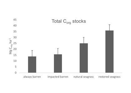
To address this knowledge gap, in the subtropics and tropics, a recent study yielded estimates of organic carbon (Corg) stocks, losses, and restoration gains from several seagrass beds around the Gulf of Mexico (GoM). GoM-wide seagrass natural Corg stocks were estimated to be ~37.2–37.5Tg Corg. A unique method involving quadruplicate sampling in naturally-occurring, restored, continually-historically barren, and previously-disturbed-now-barren sites provided the first available Corg loss measurements for subtropical-tropical seagrasses. GoM Corg losses were slow, occurring over multiple years, and differed between sites, depending on disturbance type. Mean restored seagrass bed Corg stocks exceeded those of natural seagrass beds, underscoring the importance of seagrass restoration as a viable carbon sequestration strategy. For restored seagrass areas, the older the restoration site, the greater the Corg stock.
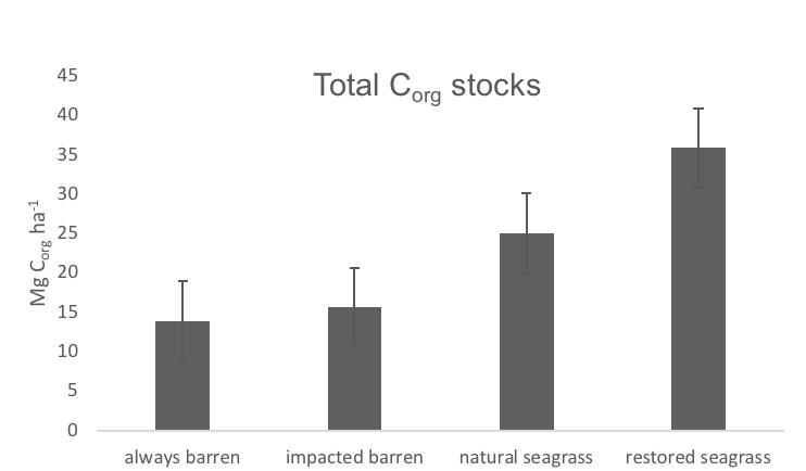
Organic carbon stocks for Gulf of Mexico sediments for the top 20 cm of sediment in always barren, impacted barren, natural seagrass, and restored seagrass sites. Natural and restored seagrass beds had significantly higher organic carbon stocks than impacted barren or always barren sediments.
Seagrass restoration appears to be an important tool for climate-change mitigation. In the USA and throughout the tropics and subtropics, restoration could reduce sedimentary carbon leakage and bolster total blue carbon stores, while facilitating increased fisheries and shoreline stability. Although well-planned and executed restoration of seagrass is more difficult than mangroves or marshes, there are >1 million hectares of degraded seagrass habitats that could be restored, which would greatly increase blue carbon sinks and support diverse marine species that rely on seagrass for habitat and food.
Authors:
Anitra Thorhaug (Yale School of Forestry)
Helen M. Poulos (Earth Sci., Wesleyan Univ.)
Jorge López-Portillo (Inecol, Mexico)
Timothy C.W. Ku (Earth Sci., Wesleyan Univ.)
Graeme P. Berlyn (Yale School of Forestry)