El Niño-Southern Oscillation (ENSO) events activate long-distance teleconnections through the atmosphere and ocean that can dramatically impact marine ecosystems along the West Coast of North America, affecting diverse organisms ranging from plankton to exploitable and protected species. Such ENSO-related changes to marine ecosystems can ultimately affect humans in many ways, including via depressed plankton and fish production, dramatic range shifts for many protected and exploited species, inaccessibility of traditionally fished resources, more prevalent harmful algal blooms, altered oxygen and pH of waters used in mariculture, and proliferation of pathogens. The principal objective of the Forecasting ENSO Impacts on Marine Ecosystems of the US West Coast workshop was to develop a scientific framework for building an ENSO-related forecast system of ecosystem indicators along the West Coast of North America, including major biological and biogeochemical responses. Attendees realized that a quantitative, biologically-focused forecast system is a much more challenging objective than forecasting the physical system alone; it requires an understanding of the ocean-atmospheric physical system and of diverse organism-level, population-level, and geochemical responses that, in aggregate, lead to altered ecosystem states.
In the tropical ocean, important advances have been made in developing both intensive observational infrastructure (Global Tropical Moored Buoy Array) and diverse dynamical and statistical models that utilize these data in ENSO forecasting. These forecasts are made widely available (e.g., NOAA’s Climate Prediction Center). The most sophisticated ENSO-forecasting efforts use global, coupled ocean-atmosphere climate models that extend ENSO-forecasting skill into seasonal climate forecasting skill for other regions, including the California Current System (CCS). However, both these measurement systems and forecast models are restricted to the physical dynamics of ENSO, rather than biotic and biogeochemical consequences.
Primary modes of influence of El Niño on marine organisms
In this brief discussion, we focus primarily on the warm (El Niño) phases of ENSO, which can have large and generally negative ecosystem consequences, although changes accompanying the cold phases (La Niña) can also be significant. We primarily address pelagic ocean processes, which merely reflect the expertise of the participants at the workshop. Physical mechanisms by which ENSO impacts the U.S. West Coast are more completely explained in Jacox et al. (this issue).
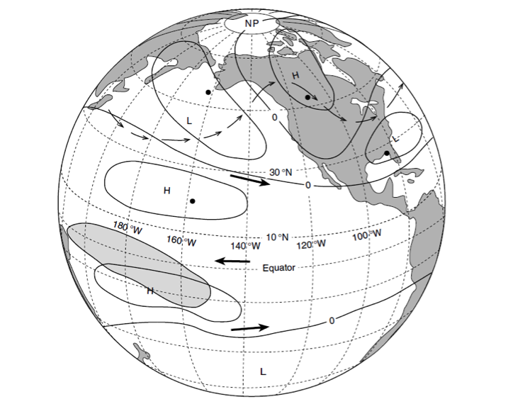
El Niño affects organisms and biogeochemistry via both local and advective processes (Figure 1). ENSO-related changes in the tropics can affect the CCS through an atmospheric teleconnection (Alexander et al. 2002) to alter local winds and surface heat fluxes, and through upper ocean processes (thermocline and sea level displacements and geostrophic currents) forced remotely by poleward propagating coastally trapped waves (CTWs) of tropical origin (Enfield and Allen 1980; Frischkencht et al. 2015; Figure 1). It is important to recognize that ecosystem effects will occur through three primary mechanisms: (1) via the direct action of altered properties like temperature, dissolved O2, and pH on the physiology and growth of marine organisms; (2) through food web effects as changes in successive trophic levels affect their predators (bottom up) or prey (top down); and (3) through changes in advection related to the combination of locally forced Ekman transport and remotely forced geostrophic currents, typically involving poleward and/or onshore transport of organisms. Advective effects can be pronounced, transporting exotic organisms into new regions and altering the food web if these imported species have significant impacts as predators, prey, competitors, parasites, or pathogens.
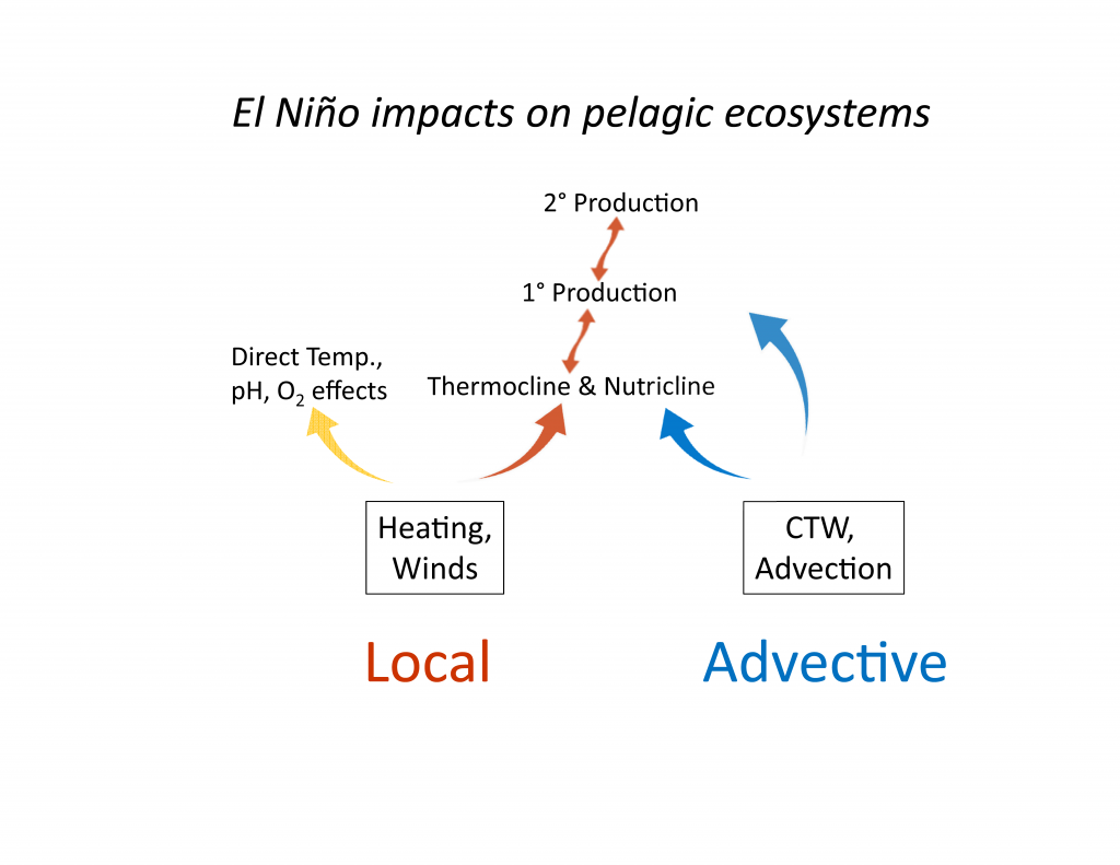
Figure 1. Schematic illustration of dominant mechanisms through which ENSO impacts biological and biogeochemical processes in the California Current System. Processes include both local effects (e.g., heat budget, winds) and advective effects. Such processes can influence organisms via: (1) (yellow arrow) direct physiological responses to changes in temperature, O2, pH, etc.; (2) (orange arrows) effects that propagate through the food web, as successive trophic levels affect their predators (bottom up, upward-facing orange arrows) or prey (top down, downward-facing orange arrows); (3) (blue arrows) direct transport effects of advection. Top predators are not included here. CTW indicates coastally trapped waves.
I. Poleward and onshore transport
Active, mobile marine fishes, seabirds, reptiles, and mammals may move into new (or away from old) habitats in the CCS as ENSO-related changes occur in the water column and render the physical-chemical characteristics and prey fields more (or less) suitable for them. Planktonic organisms are often critical prey and are, by definition, subject to geographic displacements as a consequence of altered ocean circulation that accompanies El Niño events. Most commonly, lower latitude organisms are transported poleward to higher latitudes in either surface flows or in an intensified California Undercurrent (Lynn and Bograd 2002). However, some El Niño events are accompanied by onshore flows (Simpson 1984), potentially displacing offshore organisms toward shore (Keister et al. 2005).
Two of the most celebrated examples of poleward transport come from distributions of pelagic red crabs (Pleuroncodes planipes) and the subtropical euphausiid (or krill, Nyctiphanes simplex), both of which have their primary breeding populations in waters off Baja California, Mexico (Boyd 1967; Brinton et al. 1999). Pelagic red crabs were displaced approximately 10° of latitude, from near Bahia Magdalena, Baja California, northward to Monterey, California (Glynn 1961; Longhurst 1967) during the El Niño of 1958-1959. This early event was particularly well documented because of the broad latitudinal coverage of the California Cooperative Oceanic Fisheries Investigations (CalCOFI) cruises at the time. Such El Niño-related northward displacements have been documented repeatedly over the past six decades (McClatchie et al. 2016), partly because the red crabs often strand in large windrows on beaches and are conspicuous to the general public. The normal range of the euphausiid Nyctiphanes simplex is centered at 25-30°N (Brinton et al. 1999). N. simplex has been repeatedly detected far to the north of this range during El Niño, extending at least to Cape Mendocino (40.4°N) in 1958 (Brinton 1960), to northern Oregon (46.0°N) in 1983 (Brodeur 1986), and to Newport, Oregon (44.6°N; Keister et al. 2005) and northwest Vancouver Island (50.7°N; Mackas and Galbraith 2002) in 1998. In spring of 2016, N. simplex were extremely abundant in the southern California region (M. Ohman and L. Sala, personal communication) and detected as far north as Trinidad Head (41.0°N) but not in Newport, Oregon (W. Peterson, personal communication). Sometimes such El Niño-related occurrences of subtropical species are accompanied by declines in more boreal species (e.g., Mackas and Galbraith 2002; Peterson et al. 2002), although this is not always the case.
Among the organisms displaced during El Niños, the consequences of transport of predators are poorly understood but likely significant in altering the food web. Subtropical fishes can be anomalously abundant in higher latitudes during El Niño (Hubbs 1948; Lluch-Belda et al. 2005; Pearcy and Schoener 1987; Pearcy 2002; Brodeur et al. 2006), with significant consequences for the resident food web via selective predation on prey populations.
II. Habitat compression
Many species are confined to a specific habitat that may compress during El Niño. This phenomenon has been observed repeatedly for species and processes related to coastal upwelling in the CCS. During major El Niño events, as the offshore extent of upwelled waters is reduced and becomes confined close to the coast, the zone of elevated phytoplankton (observed as Chl-a) compresses markedly to a narrow zone along the coastal boundary (e.g., Kahru and Mitchell 2000; Chavez et al. 2002). For example, during the strong El Niño spring of 1983, the temperate euphausiid Euphausia pacifica was present in low densities throughout Central and Southern California waters, but 99% of the biomass was unusually concentrated at a single location (station 80.51) very close to Point Conception, where upwelling was still pronounced (E. Brinton, personal communication). The spawning habitat of the Pacific sardine (Sardinops sagax) was narrowly restricted to the coastal boundary during El Niño 1998, but one year later during La Niña 1999, the spawning habitat extended a few hundred kilometers farther offshore (Lo et al. 2005). Market squid, Doryteuthis opalescens, show dramatically lower catches during El Niño years (Reiss et al. 2004), but in 1998, most of the catch was confined to a small region in Central California (Reiss et al. 2004). During the El Niño in spring 2016, vertical particle fluxes measured by sediment traps were reduced far offshore but remained elevated in the narrow zone of coastal upwelling very close to Point Conception (M. Stukel, personal communication).
III. Altered winds and coastal upwelling
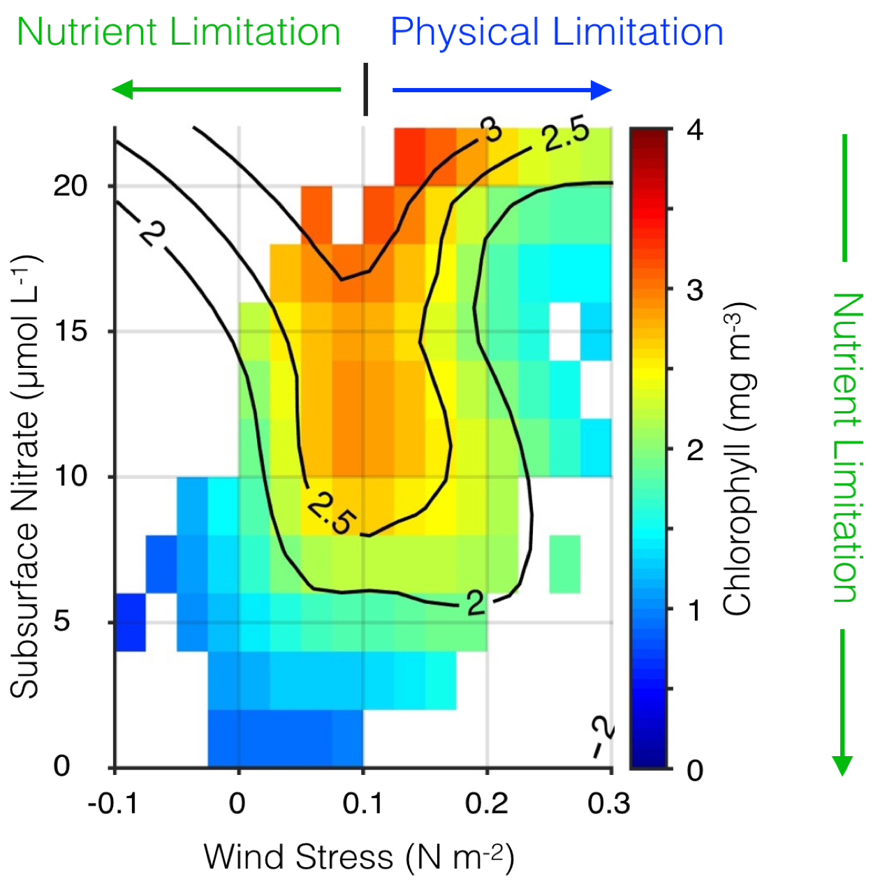
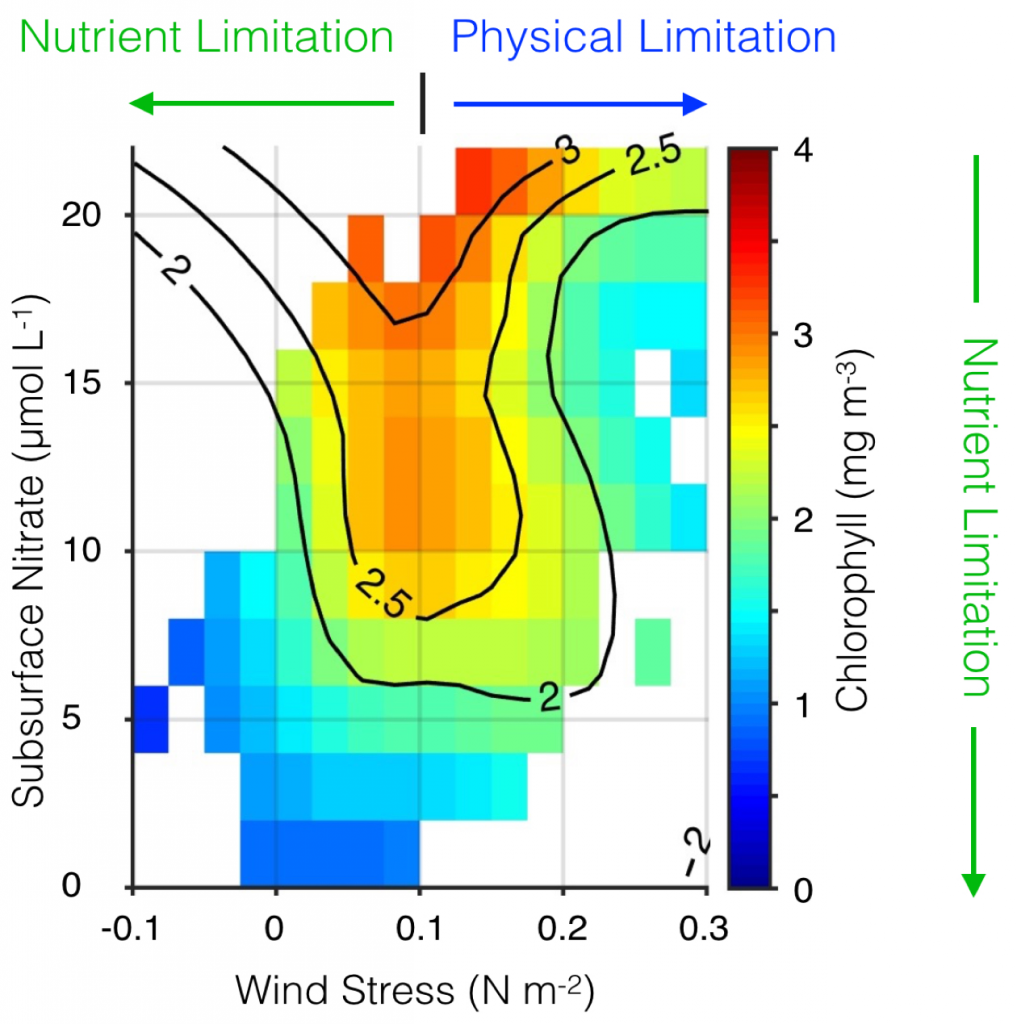
Upwelling-favorable winds along the US West Coast may decline during El Niño conditions (Hayward 2000, but see Chavez et al. 2002) and vertical transports can be reduced (Jacox et al. 2015), mainly during the winter and early spring (Black et al. 2011). Independent of any changes in density stratification (considered below), these decreased vertical velocities can lead to diminished nutrient fluxes, reduced rates of primary production, and a shift in the size composition of the plankton community to smaller phytoplankton and zooplankton (Rykaczewski and Checkley 2008). Such changes at the base of the food web can have major consequences for a sequence of consumers at higher trophic levels, as both the concentration and suitability of prey decline.
However, there are potential compensatory effects of reduced rates of upwelling. Diminished upwelling also means less introduction of CO2-rich, low-oxygen waters to coastal areas (Feely et al. 2008; Bednaršek et al. 2014), with potential benefits to organisms that are sensitive to calcium carbonate saturation state or hypoxic conditions. Furthermore, reduced upwelling implies lower Ekman transport and potentially reduced cross-shore fluxes far offshore within coastal jets and filaments (cf., Keister al. 2009).
IV. Increased stratification and deepening of nutricline
El Niño-related warming of surface waters and increased density stratification can result from advection of warmer waters and/or altered local heating. Evidence suggests that the pycnocline (Jacox et al. 2015) and nitracline (Chavez et al. 2002) deepen during stronger El Niños. This effect, independent of variations in wind stress, also leads to diminished vertical fluxes of nitrate and other limiting nutrients and suppressed rates of primary production. Decreased nitrate fluxes appear to explain elevated 15N in California Current zooplankton (Ohman et al. 2012) and decreased krill abundance (Lavaniegos and Ohman 2007; Garcia-Reyes et al. 2014) during El Niño years. For example, the 2015-16 El Niño resulted in a pronounced warming of surface waters and depressed Chl-a concentrations across a broad region of the CCS (McClatchie et al. 2016).
V. Direct physiological responses to altered temperature, dissolved O2, pH
Most organisms in the ocean—apart from some marine vertebrates—are ectothermic, meaning they have no capability to regulate their internal body temperature. Heating or cooling of the ocean therefore directly influences their rates of metabolism, growth, and mortality. Most organisms show not only high sensitivity to temperature variations but nonlinear responses. A typical temperature response curve or “thermal reaction norm” (e.g., of growth rate) is initially steeply positive with increasing temperature, followed by a narrow plateau, then abruptly declines with further increases in temperature (e.g., Eppley 1972). Different species often show different thermal reaction norms. Hence, El Niño-related temperature changes may not only alter the growth rates and abundances of organisms, but also shift the species composition of the community due to differential temperature sensitivities.
Similarly, El Niño-induced variations in dissolved oxygen concentration and pH can have marked consequences for physiological responses of planktonic and sessile benthic organisms and, for active organisms, potentially lead to migrations into or out of a suitable habitat. Interactions between variables (Boyd et al. 2010) will also lead to both winners and losers in response to major ENSO-related perturbations.
Altered parasite, predator populations, and harmful algal blooms
ENSO-related changes can favor the in situ proliferation or introduction of predators, parasites, pathogens, and harmful algal blooms. Such outbreaks can have major consequences for marine ecosystems, although some are relatively poorly studied. For example, a recent outbreak of sea star wasting disease thought to be caused by a densovirus adversely affected sea star populations at numerous locations along the West Coast (Hewson et al. 2014). While not specifically linked to El Niño, this outbreak was likely tied to warmer water temperatures. Because some sea stars are keystone predators capable of dramatically restructuring benthic communities (Paine 1966), such pathogen outbreaks are of considerable concern well beyond the sea stars themselves.
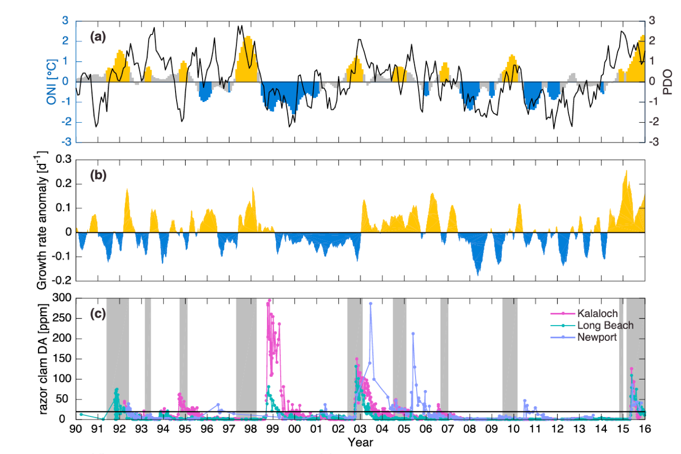
Domoic acid outbreaks, produced by some species of the diatom genus Pseudo-nitzschia, can result in closures of fisheries for razor clams, Dungeness crab, rock crab, mussels, and lobsters, resulting in significant economic losses. While the causal mechanisms leading to domoic outbreaks are under discussion (e.g., Sun et al. 2011; McCabe et al. 2016), warmer-than-normal ocean conditions in northern regions of the CCS have been linked to domoic acid accumulation in razor clams, especially when El Niño conditions coincide with the warm phase of the Pacific Decadal Oscillation (McKibben et al. 2017).
ENSO diversity, non-stationarity, and consequences of secular changes
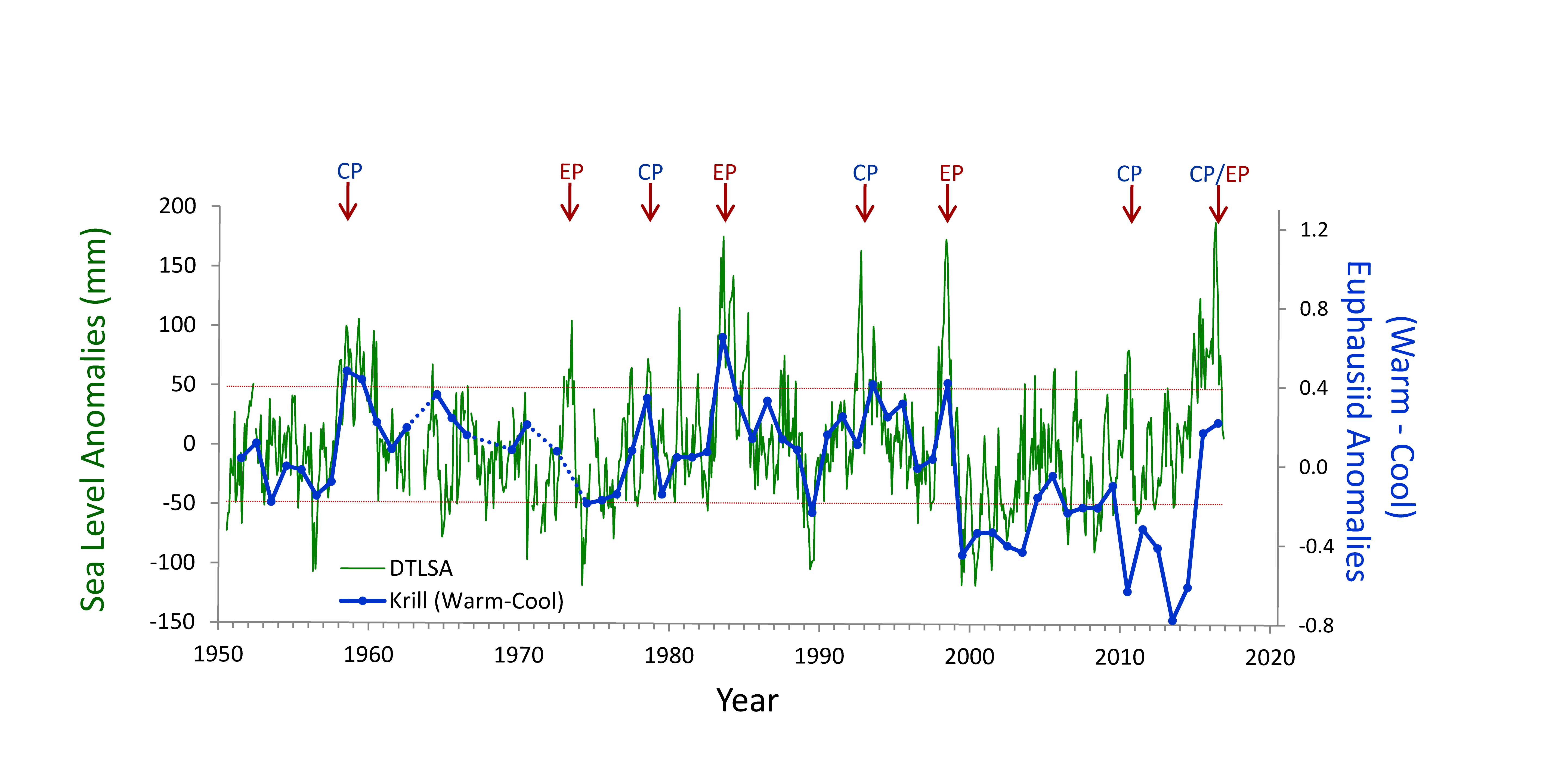
There is considerable interest in understanding the underlying dynamical drivers that lead to different El Niño events (Singh et al. 2011; Capotondi et al. 2015). Although there appears to be a continuum of El Niño expression along the equatorial Pacific, some simplify this continuum to a dichotomy between Eastern Pacific (EP) and Central Pacific (CP) events (Capotondi et al 2015). Whether EP and CP El Niños have different consequences for mid-latitude ecosystems like the California Current Ecosystem is an area of open research, but some evidence suggests that differences in timing and intensity of biological effects may exist (cf. Fisher et al. 2015). While some studies (e.g., Lee and McPhaden 2010) suggest that the frequency of CP El Niños is increasing, the evidence is not definitive (Newman et al. 2011). In addition to questions about the ecosystem consequences of El Niño diversity, there are unknowns regarding interactions between El Niño, decadal-scale variability (Chavez et al. 2002), and secular changes in climate (Figure 2, Ohman, unpubl.), which suggest a non-stationary relationship between California Current zooplankton and El Niño. An index of the dominance of warm water krill from CalCOFI sampling in Southern California shows that for the first 50 years there was a predictable positive relationship between these warm water krill and El Niño. This relationship held during both EP and CP El Niño events from 1950-2000. However, the relationship appeared to weaken after 2000. The warm water krill index was negatively correlated with the moderate El Niño of 2009-10. While the krill index again responded to the major El Niño of 2015-16 and the preceding year of warm anomalies (Bond et al. 2015; Zaba and Rudnick 2016), the magnitude of the response was not comparable to what had been seen in earlier decades. It is unclear whether such results are merely the consequence of interannual variability in the mode of El Niño propagation (Todd et al. 2011) or a change in the relationship between El Niño forcing and ecosystem responses.
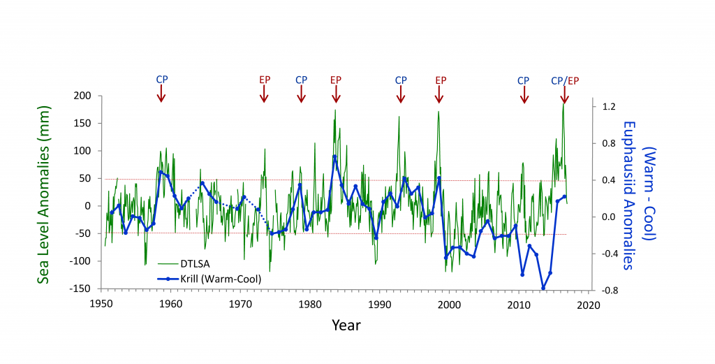
Figure 2. Covariability of California Current euphausiids (krill, blue lines) with an index of ENSO off California (de-trended sea level anomaly [DTSLA] at San Diego, green lines). Note the markedly different relationship between euphausiids and DTSLA after 2000. Sustained excursions of DTSLA exceeding one standard deviation (i.e., above upper dotted red line) are expressions of El Niño (or of the warm anomaly of 2014-2015). Red arrows indicate specific events categorized as either eastern Pacific (EP) or central Pacific (CP) El Niño events (Yu et al. 2012), apart from 2015-2016 which could be either CP or EP. The Warm-Cool euphausiid index is based on the difference in average log carbon biomass anomaly of the four dominant warm water euphausiids in the CCS minus the average anomaly of the four dominant cool water euphausiids (species affinities from Brinton and Townsend 2003). Euphausiid carbon biomass from springtime CalCOFI cruises off Southern California, lines 77-93, nighttime samples only. Dotted blue lines indicate years of no samples (Ohman, personal communication).
Conclusions
While the potential modes of El Niño influence on biological and biogeochemical processes in the CCS are numerous, not all processes are of first order consequence to all organisms. Forecasting ENSO effects on a given target species will likely focus on a limited number of governing processes. Table 1 illustrates some of the specific types of organisms susceptible to El Niño perturbations and the suspected dominant mechanism. We look forward to developing a framework for forecasting such responses in a quantitative manner.
| Ecosystem indicator | Region and season | Change during El Niño | Time scale of response | Regional ocean processes |
| Primary production | Entire CCS
winter, spring, summer |
Declines | Variable lag;
Instantaneous or time-lagged |
Reduced upwelling, nutrient fluxes; Deeper nutricline and weaker winds |
| Pseudo-nitzschia diatoms; Domoic Acid | Entire CCS
spring-summer |
Blooms |
1-3 month lag |
Elevated temperature; Altered nutrient stoichiometry |
| Copepod assemblage | NCCS
spring-summer |
Warm water species appear | Nearly instantaneous | Poleward advection; Reduced upwelling, warmer temperature |
|
Subtropical euphausiids |
SCCS spring-summer |
Increase |
Nearly instantaneous; persists beyond Niño event | Poleward advection |
| Cool water euphausiids | Entire CCS
spring-summer |
Decrease | Time-lagged | Reduced upwelling; Anomalous advection |
| Pelagic red crabs | SCCS & CCCS
winter, spring, summer |
Increase | Nearly instantaneous | Poleward advection |
| Market squid | CCCS & SCCS
winter & spring |
Collapse | Instantaneous for distribution; time-lagged for recruitment | Warmer temperature/deeper thermocline; Reduces spawning habitat |
| Pacific sardine | Entire CCS
winter-spring |
Changes in distribution;
Compression of spawning habitat |
Instantaneous for spawning and distribution, recruitment time-lagged, biomass is time-integrated | Wind stress, cross-shore transport
|
| Northern anchovy | CCCS & SCCS
winter-spring |
Changes in distribution;
Compression of spawning habitat |
Instantaneous for spawning and distribution, recruitment time-lagged, biomass is time-integrated | Reduced upwelling; Anomalous advection
|
| Juvenile salmon survival | NCCS
spring-summer |
Decrease in Pacific NW | Time-integrated | Reduce river flow, decreased food supply in ocean |
| Adult sockeye salmon
(Fraser River) |
NCCS
summer |
Return path deflected northward to Canadian waters | Time-integrated | Ocean temperature, including Ekman controls |
| Warm assemblage of mesopelagic fish | SCCS
spring (?) |
Increase | Lagged 0-3 months | Poleward and onshore advection |
| Common murre
(reproductive success) |
CCCS
winter-spring |
Decrease | Time-Lagged, time-integrated | Prey (fish) availability; Thermocline depth; Decreased upwelling? |
| Top predator reproduction and abundance | Entire CCS | Species-dependent | Time-integrated | Advection of prey, altered temperature, upwelling, mesoscale structure |
| Top predator distribution | Entire CCS | Altered geographic distributions | Instantaneous or time-lagged | Advection of prey, altered temperature, upwelling, mesoscale structure |
Authors
Mark D. Ohman (Scripps Institution of Oceanography)
Nate Mantua (NOAA Southwest Fisheries Science Center)
Julie Keister (University of Washington)
Marisol Garcia-Reyes (Farallon Institute)
Sam McClatchie (NOAA Southwest Fisheries Science Center)
References
Alexander, M. A., I. Blade, M. Newman, J. R. Lanzante, N. C. Lau, and J. D. Scott, 2002: The atmospheric bridge: The influence of ENSO teleconnections on air-sea interaction over the global oceans. Journal of Climate, 15, 2205-2231, doi: 10.1175/1520-0442(2002)015<2205:TABTIO>2.0.CO;2
Bednaršek, N., R. A. Feely, J. C. P. Reum, B. Peterson, J. Menkel, S. R. Alin, and B. Hales, 2014: Limacina helicina shell dissolution as an indicator of declining habitat suitability owing to ocean acidification in the California Current Ecosystem. Proc. Roy. Soc. B-Biolog. Sci., 281, doi: 10.1098/rspb.2014.0123.
Black, B. A., I. D. Schroeder, W. J. Sydeman, S. J. Bograd, B. K. Wells, and F. B. Schwing, 2011: Winter and summer upwelling modes and their biological importance in the California Current Ecosystem. Glob. Change Bio., 17, 2536-2545, doi: 10.1111/j.1365-2486.2011.02422.x.
Bond, N. A., M. F. Cronin, H. Freeland, and N. Mantua, 2015: Causes and impacts of the 2014 warm anomaly in the NE Pacific. Geophy. Res. Lett., 42, 3414-3420, doi: 10.1002/2015GL063306.
Boyd, C. M., 1967: The benthic and pelagic habitats of the red crab, Pleuroncodes planipes. Pacific Science, 21, 394-403.
Boyd, P. W., R. Strzepek, F. X. Fu, and D. A. Hutchins, 2010: Environmental control of open-ocean phytoplankton groups: Now and in the future. Limnol. Oceanogr., 55, 1353-1376, doi: 10.4319/lo.2010.55.3.1353.
Brinton, E., 1960: Changes in the distribution of euphausiid crustaceans in the region of the California Current. CalCOFI Reports, 7, 137-146, http://www.calcofi.org/publications/calcofireports/v07/Vol_07_Brinton.pdf.
Brinton, E., M. D. Ohman, A. W. Townsend, M. D. Knight, and A. L. Bridgeman, 1999: Euphausiids of the World Ocean. Vol. CD-ROM, MacIntosh version 1.0, UNESCO Publishing.
Brodeur, R. D., 1986: Northward displacement of the euphausiid Nyctiphanes simplex Hansen to Oregon and Washington waters following the El Niño event of 1982-83. J. Crustacean Bio., 6, 686-692, doi: 10.2307/1548382.
Brodeur, R. D., S. Ralston, R. L. Emmett, M. Trudel, T. D. Auth, and A. J. Phillips, 2006: Anomalous pelagic nekton abundance, distribution, and apparent recruitment in the northern California Current in 2004 and 2005. Geophy. Res. Lett., 33, doi:10.1029/2006gl026614.
Capotondi, A., and Coauthors, 2015: Understanding ENSO Diversity. Bull. Amer. Meteor. Soc., 96, 921-938, doi: 10.1175/BAMS-D-13-00117.1.
Chavez, F. P., and Coauthors, 2002: Biological and chemical consequences of the 1997–1998 El Niño in central California waters. Prog. Oceanogr., 54, 205-232, doi: 10.1016/S0079-6611(02)00050-2.
Enfield, D., and J. Allen, 1980: On the structure and dynamics of monthly mean sea-level anomalies along the Pacific coast of North and South America. J. Phys. Oceanogr., 10, 557–578, doi: 10.1175/1520-0485(1980)010<0557:OTSADO>2.0.CO;2.
Eppley, R. W., 1972: Temperature and phytoplankton growth in the sea. Fish. Bull, 70, 1063-1085, http://fishbull.noaa.gov/70-4/eppley.pdf.
Feely, R. A., C. L. Sabine, J. M. Hernandez-Ayon, and D. H. Ianson, B., 2008: Evidence for upwelling of corrosive “acidified” water onto the continental shelf. Science, 320, 1490-1492, doi: 10.1126/science.1155676.
Fisher J. L., W. T. Peterson, and R. R. Rykaczewski, 2015: The impact of El Niño events on the pelagic food chain in the northern California Current. Glob. Change Bio., 21, 4401–4414, doi: 10.1111/gcb.13054.
Frischknecht, M., M. Münnich, and N. Gruber, 2015: Remote versus local influence of ENSO on the California Current System, J. Geophys. Res. Oceans, 120, 1353–1374, doi:10.1002/2014JC010531.
García-Reyes, M., J. L. Largier, and W. J. Sydeman, 2014: Synoptic-scale upwelling indices and predictions of phyto-and zooplankton populations. Prog. Oceanogr., 120, 177-188, doi: 10.1016/j.pocean.2013.08.004.
Glynn, P. W., 1961: The first recorded mass stranding of pelagic red crabs, Pleuroncodes planipes, at Monterey Bay, California, since 1859, with notes on their biology. Cal. Fish Game, 47, 97-101.
Hayward, T. L., 2000: El Niño 1997-98 in the coastal waters of Southern California: a timeline of events. CalCOFI Reports, 41, 98-116, http://www.calcofi.org/publications/calcofireports/v41/Vol_41_Hayward.pdf.
Hewson, I., and Coauthors, 2014: Densovirus associated with sea-star wasting disease and mass mortality. Proc. Nat. Acad. Sci., 111, 17278-17283, doi: 0.1073/pnas.1416625111.
Hubbs, C. L., 1948: Changes in the fish fauna of western North America correlated with changes in ocean temperature, J. Mar. Res., 7, 459– 482, http://www.nativefishlab.net/library/textpdf/20041.pdf.
Jacox, M. G., J. Fiechter, A. M. Moore, and C. A. Edwards, 2015: ENSO and the California Current coastal upwelling response. J. Geophy. Res. Oceans, 120, 1691-1702, doi: 10.1002/2014JC010650.
Jacox, M.G. ….. [this issue of Variations] PLEASE ADD FULL REFERENCE
Kahru, M., E. Di Lorenzo, M. Manzano-Sarabia, and B. G. Mitchell, 2012: Spatial and temporal statistics of sea surface temperature and chlorophyll fronts in the California Current. J. Plank. Res., 34, 749-760, doi: 10.1093/plankt/fbs010.
Kahru, M., and B. G. Mitchell, 2000: Influence of the 1997-98 El Niño on the surface chlorophyll in the California Current. Geophys.Res.Lett., 27, 2937-2940, doi: 10.1029/2000GL011486
Keister, J. E., T. J. Cowles, W. T. Peterson, and C. A. Morgan, 2009: Do upwelling filaments result in predictable biological distributions in coastal upwelling ecosystems? Prog. Oceanogr., 83, 303-313, doi: 10.1016/j.pocean.2009.07.042.
Keister, J. E., T. B. Johnson, C. A. Morgan, and W. T. Peterson, 2005: Biological indicators of the timing and direction of warm-water advection during the 1997/1998 El Nino off the central Oregon coast, USA. Mar. Ecol. Prog. Ser., 295, 43-48, http://hdl.handle.net/1957/26294.
Lavaniegos, B. E., and M. D. Ohman, 2007: Coherence of long-term variations of zooplankton in two sectors of the California Current System. Prog. Oceanogr., 75, 42-69, doi: 10.1016/j.pocean.2007.07.002.
Lee, T., and M. J. McPhaden, 2010: Increasing intensity of El Nino in the central-equatorial Pacific. Geophy. Res. Lett., 37, doi: 10.1029/2010gl044007.
Lluch-Belda, D., D. B. Lluch-Cota, and S. E. Lluch-Cota, 2005: Changes in marine faunal distributions and ENSO events in the California Current. Fish. Oceanogr., 14, 458– 467, doi: 10.1111/j.1365-2419.2005.00347.x.
Lo, N. C. H., B. J. Macewicz, and D. A. Griffith, 2005: Spawning biomass of Pacific sardine (Sardinops sagax), from 1994–2004 off California. CalCOFI Reports, 46, 93-112, https://swfsc.noaa.gov/publications/TM/SWFSC/NOAA-TM-NMFS-SWFSC-463.pdf.
Longhurst, A. R., 1967: The pelagic phase of Pleuroncodes planipes Stimpson (Crustacea, Galatheidae) in the California Current. Cal. Coop. Ocean. Fish. Invest. Rep., 11, 142-154, https://decapoda.nhm.org/pdfs/29796/29796.pdf.
Lynn, R. J., and S. J. Bograd, 2002: Dynamic evolution of the 1997-1999 El Nino-La Nina cycle in the southern California Current System. Prog. Oceanogr., 54, 59-75, doi: 10.1016/S0079-6611(02)00043-5.
Mackas, D. L., and M. Galbraith, 2002: Zooplankton community composition along the inner portion of Line P during the 1997-1998 El Nino event. Prog. Oceanogr., 54, 423-437, doi: 10.1016/S0079-6611(02)00062-9.
McCabe, R. M., and Coauthors, 2016: An unprecedented coastwide toxic algal bloom linked to anomalous ocean conditions. Geophys. Res. Lett., 43, 10366-10376, doi: 10.1002/2016gl070023
McClatchie, S., and Coauthors, 2016: State of the California Current 2015-16: Comparisons with the 1997-98 El Niño. CalCOFI Reports, 57, 1-57, http://calcofi.org/publications/calcofireports/v57/Vol57-SOTCC_pages.5-61.pdf.
McKibben, S. M., W. Peterson, M. Wood, V. L. Trainer, M. Hunter, and A. E. White, 2017: Climatic regulation of the neurotoxin domoic acid. Proc. Nat. Acad. Sci., 114, 239-244, doi: 10.1073/pnas.1606798114.
Newman, M., S.-I. Shin, and M. A. Alexander, 2011: Natural variation in ENSO flavors. Geophy. Res. Lett., 38, doi:10.1029/2011GL047658.
Ohman, M. D., G. H. Rau, and P. M. Hull, 2012: Multi-decadal variations in stable N isotopes of California Current zooplankton. Deep Sea Res. I, 60, 46-55, doi: 10.1016/j.dsr.2011.11.003.
Paine, R. T., 1966: Food web complexity and species diversity. Amer. Natural., 100, 65-75, http://www.jstor.org/stable/2459379.
Pearcy, W. G., 2002: Marine nekton off Oregon and the 1997 – 98 El Niño. Prog. Oceanogr., 54, 399-403, doi: 10.1016/S0079-6611(02)00060-5.
Pearcy, W. G., and A. Schoener, 1987: Changes in the marine biota coincident with the 1982– 1983 El Niño in the northeastern subarctic Pacific Ocean. J. Geophy. Res., 92, 14,417– 14,428, doi: 10.1029/JC092iC13p14417.
Peterson, W. T., J. E. Keister, and L. R. Feinberg, 2002: The effects of the 1997-99 El Niño/La Niña events on hydrography and zooplankton off the central Oregon coast. Prog. Oceanogr., 54, 381-398, doi: 10.1016/S0079-6611(02)00059-9.
Reiss, C. S., M. R. Maxwell, J. R. Hunter, and A. Henry, 2004: Investigating environmental effects on population dynamics of Loligo opalescens in the Southern California Bight. CalCOFI Reports, 45, 87-97, http://web.calcofi.org/publications/calcofireports/v45/Vol_45_Reiss.pdf.
Rykaczewski, R. R., and D. M. Checkley, Jr., 2008: Influence of ocean winds on the pelagic ecosystem in upwelling regions. Proc. Nat. Acad. Sci., 105, 1965-1970, doi: 10.1073/pnas.0711777105.
Simpson, J. J., 1984: El Niño-induced onshore transport in the California Current during 1982-1983. Geophy. Res. Lett., 11, 241-242, doi: 10.1029/GL011i003p00233.
Singh, A., T. Delcroix, and S. Cravatte, 2011: Contrasting the flavors of El Niño-Southern Oscillation using sea surface salinity observations. J. Geophy. Res., 116, doi:10.1029/2010JC006862.
Sun, J., D. A. Hutchins, Y. Y. Feng, E. L. Seubert, D. A. Caron, and F. X. Fu, 2011: Effects of changing pCO2 and phosphate availability on domoic acid production and physiology of the marine harmful bloom diatom Pseudo-nitzschia multiseries. Limnol. Oceanogr., 56, 829-840, doi: 10.4319/lo.2011.56.3.0829.
Todd, R. E., D. L. Rudnick, R. E. Davis, and M. D. Ohman, 2011: Underwater gliders reveal rapid arrival of El Nino effects off California’s coast. Geophy. Res. Lett., 38, doi: 10.1029/2010gl046376.
Yu, J. Y., Y. H. Zou, S. T. Kim, and T. Lee, 2012: The changing impact of El Nino on US winter temperatures. Geophy. Res. Lett., 39, doi: 10.1029/2012gl052483.
Zaba, K. D., and D. L. Rudnick, 2016: The 2014–2015 warming anomaly in the Southern California Current System observed by underwater gliders. Geophy. Res. Lett., 43, 1241-1248, doi: 10.1002/2015GL067550.