Ocean Carbon & Biogeochemistry
Studying marine ecosystems and biogeochemical cycles in the face of environmental change
  • Home
  • About OCB
    • About Us
    • Scientific Breadth
      • Biological Pump
      • Changing Marine Ecosystems
      • Changing Ocean Chemistry
      • Estuarine and Coastal Carbon Fluxes
      • Ocean Carbon Uptake and Storage
      • Ocean Observatories
    • Code of Conduct
    • Get Involved
    • Project Office
    • Scientific Steering Committee
    • OCB committees
      • Ocean Time-series
      • US Biogeochemical-Argo
      • Ocean-Atmosphere Interaction
  • Activities
    • Summer Workshop
    • OCB Webinars
    • Guidelines for OCB Workshops & Activities
    • Topical Workshops
      • CMIP6 Models Workshop
      • Coastal BGS Obs with Fisheries
      • C-saw extreme events workshop
      • Ecological Forecasting – North American Coastlines
      • Expansion of BGC-Argo and Profiling Floats
      • Fish, fisheries and carbon
      • Future BioGeoSCAPES program
      • GO-BCG Scoping Workshop
      • Lateral Carbon Flux in Tidal Wetlands
      • Marine CDR Workshop
      • Ocean Nucleic Acids ‘Omics
      • Ocean-Atmosphere Interactions
      • Oceanic Methane & Nitrous Oxide
    • Small Group Activities
      • Aquatic Continuum OCB-NACP Focus Group
      • Arctic-COLORS Data Synthesis
      • BECS Benthic Ecosystem and Carbon Synthesis WG
      • Carbon Isotopes in the Ocean Workshop
      • CMIP6 WG
      • Filling the gaps air–sea carbon fluxes WG
      • Fish Carbon WG
        • Fish Carbon WG Workshop
        • Fish carbon workshop summary
      • Marine carbon dioxide removal
      • Metaproteomic Intercomparison
      • Mixotrophs & Mixotrophy WG
      • N-Fixation WG
      • Ocean Carbonate System Intercomparison Forum
      • Ocean Carbon Uptake WG
      • OOI BGC sensor WG
      • Operational Phytoplankton Observations WG
      • Phytoplankton Taxonomy WG
    • Other Workshops
    • Science Planning
      • Coastal CARbon Synthesis (CCARS)
      • North Atlantic-Arctic
    • Ocean Acidification PI Meetings
    • Training Activities
      • PACE Training Activity
  • Science Support
    • Data management and archival
    • Early Career
    • Funding Sources
    • Jobs & Postdocs
    • Meeting List
    • OCB Topical Websites
      • Ocean Fertilization
      • Trace gases
      • US IIOE-2
    • Outreach & Education
    • Promoting your science
    • Student Opportunities
    • OCB Activity Proposal Solicitations
      • Guidelines for OCB Workshops & Activities
    • Travel Support
  • Publications
    • Ocean Carbon Exchange
    • OCB Workshop Reports
    • Science Planning and Policy
    • Newsletter Archive
  • OCB Science Highlights
  • News

Using GEOTRACES data to appraise iron cycling as represented within global ocean models

Posted by mmaheigan 
· Thursday, June 23rd, 2016 

We rely on global ocean models to predict how climate change might affect the evolution of ocean productivity, acidification, and deoxygenation (1). Such platforms are also used to test hypotheses regarding the controls on ocean biogeochemical cycling and to understand past change (both on historical and geologic timescales). Ocean biogeochemistry models began with relatively simple formulations of a carbon export flux that involved restoring to observed phosphate distributions, but have more recently evolved into complex multi-element representations of the ocean. In line with our understanding that the trace micronutrient iron (Fe) limits phytoplankton productivity over large areas of the world ocean (2), most global models that aim to project future change also explicitly represent the Fe cycle.

Datasets regarding the major limiting nutrients (nitrate, phosphate, and silicate) have been available as gridded ‘climatologies’ since the early 1990s (3). This has greatly facilitated the development and evaluation of modelled distributions over the past two decades. However, over this period there has been little comprehensive evaluation of how different models represent the ocean Fe cycle. Over recent years, there has been a marked increase in the availability of iron measurements in the ocean (4), largely driven by the international GEOTRACES effort to conduct full depth, basin-scale surveys. This led us to initiate the first-ever attempt to critically compare a range of global ocean iron models against the largest global datasets, as well as against the newly emerging ocean section data (5).

The Fe Model Intercomparison Project (FeMIP) sought to be as inclusive as possible in this first step and therefore did not seek to standardize the underlying ocean circulation or external inputs. Instead, we simply asked each of the thirteen models to provide their best representation of dissolved iron in three dimensions at monthly resolution. We then compared these models against each other, a global iron database of over 20,000 observations and against five unique basin-scale sections from the GEOTRACES intermediate data product 2014 (IDP2014) (6).

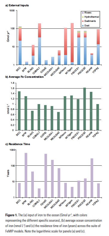
Firstly, it is apparent that even when the underlying iron cycles of the different models are evaluated, a substantial degree of inter-model discord exists. The total iron input varies from around 2 to 200 Gmol yr-1 across the thirteen models (Fig. 1a). Even for ‘well known’ sources like atmospheric deposition, the inter-model variability is around an order of magnitude. On the other hand, the average concentrations of dissolved Fe between the models is much less variable and ranges from 0.35 to 0.81 nmol L-1 (Fig. 1b), or an average of 0.58±0.14 nmol L-1. This apparent constancy reflects an initial view of the ocean Fe cycle in which interior Fe concentrations were held at a quasi-constant value of 0.6 nmol L-1 assuming a constant concentration of Fe-binding ligands (7). Thus the FeMIP models are balancing widely varying Fe input fluxes against relatively constant overall Fe concentrations by tuning the Fe scavenging rate, which is a crucial but poorly known parameter. This results in residence times for Fe that range from <5 to >500 years across the FeMIP models (Fig 1c). This difference is important, as it represents substantial inter-model deviation concerning the timescales over which the different models respond to a perturbation in Fe supply.

When compared statistically against the global dataset, similar levels of variability arise. Some models display correlation coefficients of >0.5, whereas others are slightly anti-correlated. When the FeMIP models are compared against the five GEOTRACES sections, it becomes apparent that those models that represent the newly emerging features of the iron cycle perform much better. For instance, having Fe scavenging rates that vary in space and time, including variable Fe:carbon (C) stoichiometry, multiple Fe sources, and representing ligand concentrations in a dynamic manner, all act to improve the representation of different observed features in the models. Importantly, the IDP2014 provided the opportunity to demonstrate that the issues at hand were specific to Fe, since the models could represent the observed distributions of major nutrients with a much greater degree of skill (5).

The next stage of FeMIP will be a deeper comparison of the processes themselves. Of particular interest is whether GEOTRACES datasets can provide broader assessments of the rates of Fe scavenging – e.g., using other particle-reactive, non-biological tracers such as thorium (8, 9). Equally, the emerging database of GEOTRACES process studies provides an important opportunity to appraise the way different models represent biological iron cycling and in particular, the often-observed importance of recycled and remineralized sources of Fe (10, 11). Finally, the new GEOTRACES intermediate data product 2017 will also facilitate further evaluation of models, providing new section data from the Atlantic, Pacific and Arctic Oceans.

Author

Alessandro Tagliabue (Dept. of Earth, Ocean and Ecological Sciences, School of Environmental Sciences, University of Liverpool)

References

1. L. Bopp et al., Biogeosci. 10(10), 6225-6245, doi:10.5194/bg-10-6225-2013 (2013).
2. C. M. Moore et al., Nature Geosci., doi:10.1038/ngeo1765 (2013).
3. S. Levitus et al., Prog. Oceanogr. 31(3), 245-273, doi:10.1016/0079-6611(93)90003-v (1993).
4. A. Tagliabue et al., Biogeosci. 9(6), 2333-2349, doi:10.5194/bg-9-2333-2012 (2012).
5. A. Tagliabue, A. et al., Glob. Biogeochem. Cycles, doi:10.1002/2015gb005289 (2016).
6. E. Mawji et al., Marine Chem. 177, 1-8. doi:10.1016/j. marchem.2015.04.005 (2015).
7. K. S. Johnson, R. M. Gordon, K. H. Coale, Marine Chem. 57(3-4), 137-161, doi:10.1016/s0304-4203(97)00043-1 (1997).
8. C. T. Hayes et al., Geochim. Cosmochim. Acta 169, 1-16, doi:10.1016/j.gca.2015.07.019 (2015).
9. N. Rogan et al., Geophys. Res. Lett. 43(6), 2732-2740. doi:10.1002/2016gl067905 (2016).
10. P. W. Boyd et al., Glob. Biogeochem. Cycles 29(7), 1028-1043, doi:10.1002/2014gb005014 (2015).
11. R. F. Strzepek et al., Glob. Biogeochem. Cycles 19(4), GB4S26, doi:10.1029/2005gb002490 (2005).

Filter by Keyword

234Th disequilibrium abundance acidification africa air-sea flux air-sea interactions air-sea interface algae alkalinity allometry ammonium AMOC anoxia anoxic Antarctic anthro impacts anthropogenic carbon aquaculture aragonite saturation arctic Argo argon arsenic artificial seawater Atlantic Atlantic modeling atmospheric carbon atmospheric CO2 atmospheric nitrogen deposition authigenic carbonates autonomous platforms bacteria BATS BCG Argo benthic bgc argo bio-go-ship bio-optical bioavailability biogeochemical cycles biogeochemical cycling biogeochemical models biogeochemistry Biological Essential Ocean Variables biological pump biological uptake biophysics bloom blooms blue carbon bottom water boundary layer buffer capacity C14 CaCO3 calcification calcite calcium carbonate carbon-climate feedback carbon-sulfur coupling carbon budget carbon cycle carbon dioxide carbon export carbon sequestration carbon storage Caribbean CCA CCS changi changing marine ecosystems changing marine environments changing ocean chemistry chemical oceanographic data chemical speciation chemoautotroph chesapeake bay chl a chlorophyll circulation climate change climate variability CO2 CO2YS coastal darkening coastal ocean cobalt Coccolithophores community composition conservation cooling effect copepod coral reefs CTD currents cyclone data data access data management data product Data standards DCM dead zone decadal trends decomposers decomposition deep convection deep ocean deep sea coral deoxygenation depth diagenesis diatoms DIC diel migration diffusion dimethylsulfide dinoflagellate discrete measurements dissolved inorganic carbon dissolved organic carbon DOC DOM domoic acid dust DVM earth system models ecology ecosystems ecosystem state eddy Education Ekman transport emissions ENSO enzyme equatorial regions error ESM estuarine and coastal carbon estuarine and coastal carbon fluxes estuary euphotic zone eutrophication evolution export export fluxes export production EXPORTS extreme events extreme weather events faecal pellets filter feeders filtration rates fire fish Fish carbon fisheries floats fluid dynamics fluorescence food webs forage fish forams freshening freshwater frontal zone fronts functional role future oceans geochemistry geoengineering geologic time GEOTRACES glaciers gliders global carbon budget global ocean global warming go-ship grazing greenhouse gas Greenland groundwater Gulf of Maine Gulf of Mexico Gulf Stream gyre harmful algal bloom high latitude human food human impact hurricane hydrogen hydrothermal hypoxia ice age ice cores ice cover industrial onset inverse circulation ions iron iron fertilization isotopes jellies katabatic winds kelvin waves krill kuroshio laboratory vs field land-ocean continuum larvaceans lateral transport LGM lidar ligands light light attenuation lipids mangroves marine carbon cycle marine heatwave marine particles marine snowfall marshes Mediterranean meltwater mesopelagic mesoscale metagenome metals methane methods microbes microlayer microorganisms microscale microzooplankton midwater mixed layer mixed layers mixing mixotrophy modeling models mode water molecular diffusion MPT multi-decade n2o NAAMES NASA NCP net community production net primary productivity new ocean state new technology Niskin bottle nitrate nitrogen nitrogen fixation nitrous oxide north atlantic north pacific nuclear war nutricline nutrient budget nutrient cycling nutrient limitation nutrients OA ocean-atmosphere ocean acidification ocean acidification data ocean carbon uptake and storage ocean color ocean observatories ocean warming ODZ oligotrophic omics OMZ open ocean optics organic particles oscillation overturning circulation oxygen pacific paleoceanography particle flux particles pCO2 PDO peat pelagic PETM pH phenology phosphorus photosynthesis physical processes physiology phytoplankton PIC plankton POC polar regions pollutants precipitation predation prediction primary production primary productivity Prochlorococcus proteins pteropods pycnocline radioisotopes remineralization remote sensing repeat hydrography residence time resource management respiration resuspension rivers rocky shore Rossby waves Ross Sea ROV salinity salt marsh satell satellite scale seafloor seagrass sea ice sea level rise seasonal patterns seasonal trends sea spray seaweed sediments sensors shelf system shells ship-based observations shorelines silicate silicon cycle sinking particles size SOCCOM soil carbon southern ocean south pacific spatial covariations speciation SST stoichiometry subduction submesoscale subpolar subtropical sulfate surf surface surface ocean Synechococcus teleconnections temperate temperature temporal covariations thermocline thermodynamics thermohaline thorium tidal time-series time of emergence top predators total alkalinity trace elements trace metals trait-based transfer efficiency transient features Tris trophic transfer tropical turbulence twilight zone upper ocean upper water column upwelling US CLIVAR validation velocity gradient ventilation vertical flux vertical migration vertical transport volcano warming water clarity water quality waves western boundary currents wetlands winter mixing world ocean compilation zooplankton

Copyright © 2023 - OCB Project Office, Woods Hole Oceanographic Institution, 266 Woods Hole Rd, MS #25, Woods Hole, MA 02543 USA Phone: 508-289-2838  •  Fax: 508-457-2193  •  Email: ocb_news@us-ocb.org

link to nsflink to noaalink to WHOI

Funding for the Ocean Carbon & Biogeochemistry Project Office is provided by the National Science Foundation (NSF) and the National Aeronautics and Space Administration (NASA). The OCB Project Office is housed at the Woods Hole Oceanographic Institution.