Have you ever wondered what life would be like if you could write and run complex biogeochemical models easily and conveniently in Python? Wonder no more. In a paper published in J. Adv. Model. Earth Syst., Samar Khatiwala (2025; see reference below) describes tmm4py, a new software to enable efficient, global scale biogeochemical modelling in Python.
tmm4py is based on the Transport Matrix Method (TMM), an efficient numerical scheme for “offline” simulation of tracers driven by circulations from state-of-the-art physical models and state estimates. tmm4py exposes this functionality in Python, providing the tools needed to implement complex models in pure Python using standard modules such as NumPy, and run them interactively on hardware ranging from laptops to supercomputers. No knowledge of parallel computing required! tmm4py even extends the interactivity to models written in Fortran, allowing the many existing models coupled to the TMM, e.g., MITgcm, to be used from the familiar comfort of Python. Whether you’re a seasoned modeler, just want to try out an idea, or illustrate a concept in your teaching, tmm4py is designed to make biogeochemical modeling more widely accessible.
Download the code from: https://github.com/samarkhatiwala/tmm
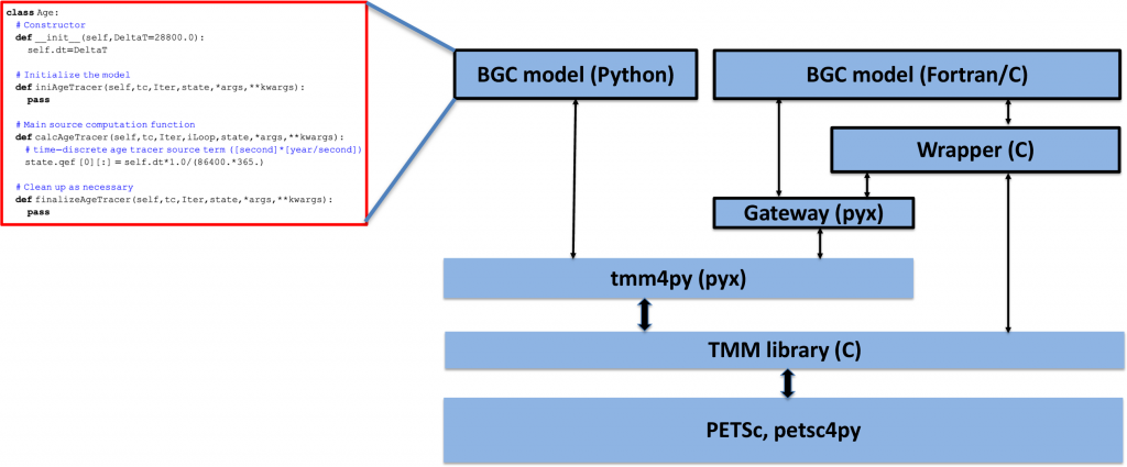
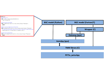
Figure: Schematic illustrating the structure of tmm4py and its relationship with the various libraries and components it is built on or interacts with. Outlined boxes represent user‐supplied code (such as the “Hello World” example of the ideal age tracer shown on the left). Other low-level libraries on which tmm4py depends, for example, BLAS and LAPACK for linear algebra, MPI for parallel communication, and CUDA for GPUs, are not shown.
Author
Samar Khatiwala (Waseda Univ)
Joint Science Highlight with GEOTRACES.