modeling :: Ocean Carbon & Biogeochemistry

Studying marine ecosystems and biogeochemical cycles in the face of environmental change

Archive for modeling – Page 4

Estuarine sediment resuspension drives non-local impacts on biogeochemistry

Posted by mmaheigan

· Friday, September 18th, 2020

Sediment processes, including resuspension and transport, affect water quality in estuaries by altering light attenuation, primary productivity, and organic matter remineralization, which then influence oxygen and nitrogen dynamics. In a recent paper published in Estuaries and Coasts, the authors quantified the degree to which sediment resuspension and transport affected estuarine biogeochemistry by implementing a coupled hydrodynamic-sediment transport-biogeochemical model of the Chesapeake Bay. By comparing summertime model runs that either included or neglected seabed resuspension, the study revealed that resuspension increased light attenuation, especially in the northernmost portion of the Bay, which subsequently shifted primary production downstream (Figure 1). Resuspension also increased remineralization in the central Bay, which experienced higher organic matter concentrations due to the downstream shift in primary productivity. When combined with estuarine circulation, these resuspension-induced shifts caused oxygen to increase and ammonium to increase throughout the Bay in the bottom portion of the water column. Averaged over the channel, resuspension decreased oxygen by ~25% and increased ammonium by ~50% for the bottom water column. Changes due to resuspension were of the same order of magnitude as, and generally exceeded, short-term variations within individual summers, as well as interannual variability between wet and dry years. This work highlights the importance of a localized process like sediment resuspension and its capacity to drive biogeochemical variations on larger spatial scales. Documenting the spatiotemporal footprint of these processes is critical for understanding and predicting the response of estuarine and coastal systems to environmental changes, and for informing management efforts.

Figure 1: Schematic of how resuspension affects biogeochemical processes based on HydroBioSed model estimates for Chesapeake Bay.

Authors:
Julia M. Moriarty (University of Colorado Boulder)
Marjorie A. M. Friedrichs (Virginia Institute of Marine Science)
Courtney K. Harris (Virginia Institute of Marine Science)

Also see the Geobites piece “Muddy waters lead to decreased oxygen in Chesapeake Bay” on this publication, by Hadley McIntosh Marcek

A close-up view of biomass controls in Southern Ocean eddies

Posted by mmaheigan

· Thursday, August 20th, 2020

Southern Ocean biological productivity is instrumental in regulating the global carbon cycle. Previous correlative studies associated widespread mesoscale activity with anomalous chlorophyll levels. However, eddies simultaneously modify both the physical and biogeochemical environments via several competing pathways, making it difficult to discern which mechanisms are responsible for the observed biological anomalies within them. Two recently published papers track Southern Ocean eddies in a global, eddy-resolving, 3-D ocean simulation. By closely examining eddy-induced perturbations to phytoplankton populations, the authors are able to explicitly link eddies to co-located biological anomalies through an underlying mechanistic framework.

Figure caption: Simulated Southern Ocean eddies modify phytoplankton division rates in different directions of depending on the polarity of the eddy and background seasonal conditions. During summer anticyclones (top right panel) deliver extra iron from depth via eddy-induced Ekman pumping and fuel faster phytoplankton division rates. During winter (bottom right panel) the extra iron supply is eclipsed by deeper mixed layer depths and elevated light limitation resulting in slower division rates. The opposite occurs in cyclones.

In the first paper, the authors observe that eddies primarily affect phytoplankton division rates by modifying the supply of iron via eddy-induced Ekman pumping. This results in elevated iron and faster phytoplankton division rates in anticyclones throughout most of the year. However, during deep mixing winter periods, exacerbated light stress driven by anomalously deep mixing in anticyclones can dominate elevated iron and drive division rates down. The opposite response occurs in cyclones.

The second paper tracks how eddy-modified division rates combine with eddy-modified loss rates and physical transport to produce anomalous biomass accumulation. The biomass anomaly is highly variable, but can exhibit an intense seasonal cycle, in which cyclones and anticyclones consistently modify biomass in different directions. This cycle is most apparent in the South Pacific sector of the Antarctic Circumpolar Current, a deep mixing region where the largest biomass anomalies are driven by biological mechanisms rather than lateral transport mechanisms such as eddy stirring or propagation.

It is important to remember that the correlation between chlorophyll and eddy activity observable from space can result from a variety of physical and biological mechanisms. Understanding the nuances of how these mechanisms change regionally and seasonally is integral in both scaling up local observations and parameterizing coarser, non-eddy resolving general circulation models with embedded biogeochemistry.

Authors:
Tyler Rohr (Australian Antarctic Partnership Program, previously at MIT/WHOI)
Cheryl Harrison (University of Texas Rio Grande Valley)
Matthew Long (National Center for Atmospheric Research)
Peter Gaube (University of Washington)
Scott Doney (University of Virginia)

Multiyear predictions of ocean acidification in the California Current System

Posted by mmaheigan

· Thursday, August 20th, 2020

The California Current System is a highly productive coastal upwelling region that supports commercial fisheries valued at $6 billion/year. These fisheries are supported by upwelled waters, which are rich in nutrients and serve as a natural fertilizer for phytoplankton. Due to remineralization of organic matter at depth, these upwelled waters also contain large amounts of dissolved inorganic carbon, causing local conditions to be more acidic than the open ocean. This natural acidity, compounded by the dissolution of anthropogenic CO₂ into coastal waters, creates corrosive conditions for shell-forming organisms, including commercial fishery species.

A recent study in Nature Communications showcases the potential for climate models to skillfully predict variations in surface pH—thus ocean acidification—in the California Current System. The authors evaluate retrospective predictions of ocean acidity made by a global Earth System Model set up similarly to a weather forecasting system. The forecasting system can already predict variations in observed surface pH fourteen months in advance, but has the potential to predict surface pH up to five years in advance with better initializations of dissolved inorganic carbon (Figure 1). Skillful predictions are mostly driven by the model’s initialization and subsequent transport of dissolved inorganic carbon throughout the North Pacific basin.

Figure 1. Forecast of annual surface pH anomalies in the California Current Large Marine Ecosystem for 2020. Red colors denote anomalously basic conditions for the given location and blue colors indicate anomalously acidic conditions.

These results demonstrate, for the first time, the feasibility of using climate models to make multiyear predictions of surface pH in the California Current. Output from this global prediction system could serve as boundary conditions for high-resolution models of the California Current to improve prediction time scale and ultimately help inform management decisions for vulnerable and valuable shellfisheries.

Authors:
Riley X. Brady (University of Colorado Boulder)
Nicole S. Lovenduski (University of Colorado Boulder)
Stephen G. Yeager (National Center for Atmospheric Research)
Matthew C. Long (National Center for Atmospheric Research)
Keith Lindsay (National Center for Atmospheric Research)

Blue hole in the South China Sea reveals ancient carbon

Posted by mmaheigan

· Wednesday, July 8th, 2020

Blue holes are unique depositional environments that are formed within carbonate platforms. Due to an enclosed geomorphology that restricts water exchange, blue hole ecosystems are typically characterized by steep biogeochemical gradients and distinctive microbial communities. For the past three decades, studies have described vertical gradients in physical, chemical, and biological parameters that typify blue hole water columns, but their elemental cycles, particularly carbon, remain poorly understood.

Figure 1. Aerial photo of the Yongle Blue Hole in the South China Sea (Credit: P. Yao et al./JGR Biogeosciences)

In July 2016, the Yongle Blue Hole (YBH) was discovered to be the deepest known blue hole on Earth (~300 m). YBH is located in the Xisha Islands of the South China Sea. The unique features and ease of accessibility make YBH an ideal natural laboratory for studying carbon cycling in marine anoxic systems. In a recent study published in JGR Biogeosciences, the authors reported extremely low concentrations of dissolved organic carbon (DOC) (e.g., 22 µM) and very high concentrations of dissolved inorganic carbon (DIC) (e.g., 3,090 µM) in YBH deep waters. Radiocarbon dating revealed that the YBH DOC and DIC were unusually old, yielding ages (6,810 and 8270 years BP, respectively) that are much more typical of open ocean deep water. Based on H₂S and microbial community composition profiles, the authors concluded that sharp redox gradients and a high abundance of sulfur cycling bacteria were likely responsible for much of the DOC consumption in YBH. The unusually low concentrations and old DOC ages in the relatively shallow YBH suggest short-term cycling of recalcitrant DOC in oceanic waters, which has been recognized as a long-term microbial carbon sink in the global ocean. The stoichiometry of DIC and total alkalinity changes suggested that the accumulation of DIC in the deep layer of the YBH was largely derived from both the dissolution of carbonate and OC decomposition through sulfate reduction. However, the role of carbonate dissolution from the walls of the blue hole in affecting the old ages of carbon in this system remain uncertain, yet there appears to no evidence of subterranean freshwater into the bottom waters of the blue hole. In the face of expanding oxygen minimum zones and anthropogenically-induced coastal hypoxia, blue holes such as YBH can provide an accessible natural laboratory in which to study the microbial and biogeochemical features that typify these low-oxygen systems.

Authors:
Peng Yao (Ocean University of China)
Thomas S. Bianchi (University of Florida)
Xuchen Wang (Ocean University of China)
Zuosheng Yang (Ocean University of China)
Zhigang Yu (Ocean University of China)

Global change impacts soil carbon storage in blue carbon ecosystems

Posted by mmaheigan

· Wednesday, May 20th, 2020

Vegetated coastal “blue carbon” ecosystems, including sea grasses, mangroves, and salt marshes, provide valuable ecosystem services such as carbon sequestration, storm protection, critical habitat, etc.. Many of these services are supported by the ability of blue carbon ecosystems to accumulate soil organic carbon over thousands of years. Rapidly changing climate and environmental conditions will impact decomposition and thus the global reservoir of organic carbon in coastal soils. A recent Perspective article published in Nature Geoscience focused on the biogeochemical factors affecting decomposition in coastal soils, such as mineral protection, redox zonation, water content and movement, and plant-microbe interactions. The authors explored the spatial and temporal scales of these decomposition mechanisms and developed a conceptual framework to characterize how they may respond to environmental disturbances such as land-use change, nutrient loading, warming, and sea-level rise.

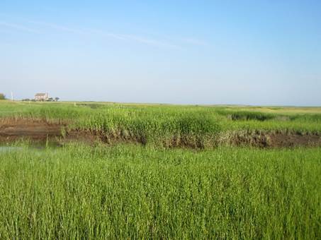
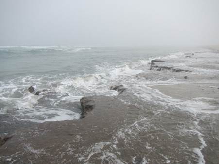
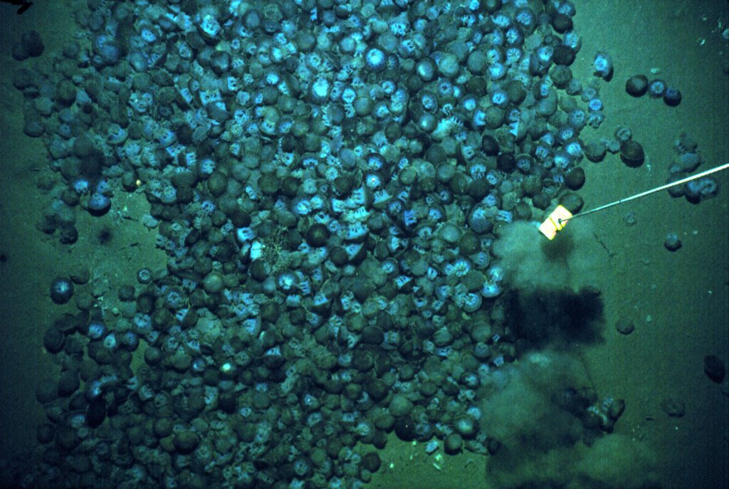
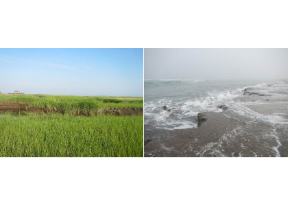
Figure caption: Temperate salt marshes (MA, USA). Healthy salt marshes have lush stands of grasses (top). Storms can expose peat deposits that have been buried for thousands of years (bottom). The fate of this soil carbon is unknown, but some fraction will be respired by microbes and returned to the atmosphere as CO₂.

Improved estimates of soil organic carbon in blue carbon systems will require better characterization of these processes from sustained data sets. Furthermore, incorporation of these decomposition mechanisms into ecosystem evolution models will improve our capacity to quantify and predict changes in these soil carbon reservoirs, which could facilitate their inclusion in global budgets and management tools.

Temperate salt marshes (MA, USA). Healthy salt marshes have lush stands of grasses (left/top). Storms can expose peat deposits that have been buried for thousands of years (right/bottom). The fate of this soil carbon is unknown, but some fraction will be respired by microbes and returned to the atmosphere as CO₂.

Authors:
Amanda C Spivak (University of Georgia)
Jon Sanderman (Woods Hole Research Center)
Jennifer Bowen (Northeastern University)
Elizabeth A. Canuel (Virginia Institute of Marine Science)
Charles S Hopkinson (University of Georgia)

Little big exporters

Posted by mmaheigan

· Wednesday, April 8th, 2020

In the Southern Ocean, coccolithophores are thought to account for a major fraction of marine carbonate production and export to the deep sea. Despite their importance in the ocean carbon cycle, we lack fundamental information about Southern Ocean coccolithophore abundance, species composition, and contribution to carbonate export.

Figure caption: Heliscosphaera carteri (left), Coccolithus pelagicus (right) and Emiliania huxleyi (bottom right, partially behind C. pelagicus) coccospheres retrieved from the subantarctic waters south of Tasmania. Image Ruth Eriksen, courtesy AAD EMU.

A recent study in Biogeosciences has generated annual observations of coccolithophore species composition and contribution to calcium carbonate fluxes at two sites that are representative of a large portion of the Subantarctic zone. Coccolithophores account for roughly half of the annual calcium carbonate exported to the deep sea. Notably, it is not the most abundant species (Emiliania huxleyi), but rather the less abundant and larger species (e.g. Calcidiscus leptoporus, Helicosphaera carteri and Coccolithus pelagicus) that make the greatest contribution to carbonate export to the deep sea. Since these larger species exhibit substantially different ecological traits from the opportunistic E. huxleyi, predictions of future response of Southern Ocean coccolithophore communities should not be based on the physiological results from experiments with E. huxleyi. Rather, new physiological response experiments of those less abundant, larger coccolithophore species are urgently needed to constrain responses of these important carbonate exporters to environmental change in the Southern Ocean. This study underscores the importance of phytoplankton ecological traits on the regulation of the marine carbon cycle and emphasizes the need for more species-specific studies to improve predictions of marine ecosystem response to ongoing climate change.

Authors
Andrés S. Rigual Hernández (Universidad de Salamanca)
Thomas W. Trull (CSIRO and ACE CRC)
Scott D. Nodder (NIWA)
José A. Flores (Universidad de Salamanca)
Helen Bostock (University of Queensland,)
Fátima Abrantes (Portuguese Institute for Sea and Atmosphere and CCMAR)
Ruth S. Eriksen (CSIRO and IMAS)
Francisco J. Sierro (Universidad de Salamanca)
Diana M. Davies (CSIRO and ACE CRC)
Anne-Marie Ballegeer (Universidad de Salamanca)
Miguel A. Fuertes (Universidad de Salamanca)
Lisa C. Northcote (NIWA)

Tiny, but effective: Gelatinous zooplankton and the ocean biological carbon pump

Posted by mmaheigan

· Wednesday, March 25th, 2020

Barely visible to the naked eye, gelatinous zooplankton play important roles in marine food webs. Cnidaria, Ctenophora, and Urochordata are omnipresent and provide important food sources for many more highly developed marine organisms. These small, nearly transparent organisms also transport large quantities of “jelly-carbon” from the upper ocean to depth. A recent study in Global Biogeochemical Cycles focused on quantifying the gelatinous zooplankton contribution to the ocean carbon cycle.

Figure 1. Processes and pathways or gelatinous carbon transfer to the deep ocean.

Using >90,000 data points (1934 to 2011) from the Jellyfish Database Initiative (JeDI), the authors compiled global estimates of jellyfish biomass, production, vertical migration, and jelly carbon transfer efficiency. Despite their small biomass relative to the total mass of organisms living in the upper ocean, their rapid, highly efficient sinking makes them a globally significant source of organic carbon for deep-ocean ecosystems, with 43-48% of their upper ocean production reaching 2000 m, which translates into 0.016 Pg C yr^-1.

Figure 2. Mass deposition event of jellyfish at 3500 m in the Arabian Sea (Billett et al. 2006).

Sediment trap data have suggested that carbon transport associated with large, episodic gelatinous blooms in localized open ocean and continental shelf regions could often exceed phytodetrital sources, in particular instances. These mass deposition events and their contributions to deep carbon export must be taken into account in models to better characterize marine ecosystems and reduce uncertainties in our understanding of the ocean’s role in the global carbon cycle.

Links:

Jellyfish Database Initiative http://jedi.nceas.ucsb.edu, http://jedi.nceas.ucsb.edu-dmo.org/dataset/526852 )

Authors:
Mario Lebrato (Christian‐Albrechts‐University Kiel and Bazaruto Center for Scientific Studies, Mozambique)
Markus Pahlow (GEOMAR)
Jessica R. Frost (South Florida Water Management District)
Marie Küter (Christian‐Albrechts‐University Kiel)
Pedro de Jesus Mendes (Marine and Environmental Scientific and Technological Solutions, Germany)
Juan‐Carlos Molinero (GEOMAR)
Andreas Oschlies (GEOMAR)

Chasing Sargassum in the Atlantic Ocean

Posted by mmaheigan

· Wednesday, March 25th, 2020

The pelagic brown alga Sargassum forms a habitat that hosts a rich diversity of life, including other algae, crustaceans, fish, turtles, and birds in both the Gulf of Mexico and the area of the Atlantic Ocean known as the Sargasso Sea. However, high abundances of Sargassum have been appearing in the tropical Atlantic, in some cases 3,000 miles away from the Sargasso Sea. This is a new phenomenon. Nearly every year since 2011, thick mats of Sargassum have blanketed the coastlines of many countries in tropical Africa and the Americas. When masses of Sargassum wash ashore, the seaweed rots, attracts insects, and repels beachgoers, with adverse ecological and socioeconomic effects. A new study in Progress in Oceanography sheds light on the mystery.

Figure 1. The hypothesized route of Sargasso Sea Sargassum to the tropical Atlantic and the Caribbean Sea. The solid black lines indicate the climatological surface flow, the dashed black lines indicate areas where there was variability from the average conditions.

The authors analyzed reams of satellite data and used computer models of the Earth’s winds and ocean currents to try to understand why these large mats started to arrive in coastal areas in 2011. A strengthening and southward shift of the westerlies in the winter of 2009-2010 caused ocean currents to move the Sargassum toward the Iberian Peninsula, then southward in the Canary Current along Africa, where it entered the tropics by the middle of 2010 (Figure 1). The tropical Atlantic provided ample sunlight, warmer sea temperatures, and nutrients for the algae to flourish. In 2011, Sargassum spread across the entire tropical Atlantic in a massive belt north of the Equator, along the Intertropical Convergence Zone (ITCZ), and these blooms have appeared nearly every year since. Utilizing international oceanographic studies done in the Atlantic since the 1960s, and multiple satellite sensors combined with Sargassum distribution patterns, the authors discovered that the trade winds aggregate the Sargassum under the ITCZ and mix the water deep enough to bring new nutrients to the surface and sustain the bloom.

Improved understanding and predictive capacity of Sargassum bloom occurrence will help us better constrain and quantify its impacts on our ecosystems, which can inform management of valuable fisheries and protected species.

Authors:
Elizabeth Johns (NOAA AMOL)
Rick Lumpkin (NOAA AMOL)
Nathan Putman (LGL Ecological Research Associates)
Ryan Smith (NOAA AMOL)
Frank Muller-Karger (University of South Florida)
Digna Rueda-Roa (University of South Florida)
Chuanmin Hu (University of South Florida)
Mengqiu Wang (University of South Florida)
Maureen Brooks (University of Maryland Center for Environmental Science)
Lewis Gramer (NOAA AMOL and University of Miami)
Francisco Werner (NOAA Fisheries)

Can phytoplankton help us determine ocean iron bioavailability?

Posted by mmaheigan

· Wednesday, March 11th, 2020

Iron (Fe) is a key element to sustaining life, but it is present at extremely low concentrations in seawater. This scarcity limits phytoplankton growth in large swaths of the global ocean, with implications for marine food webs and carbon cycling. The acquisition of Fe by phytoplankton is an important process that mediates the movement of carbon to the deep ocean and across trophic levels. It is a challenge to evaluate the ability of marine phytoplankton to obtain Fe from seawater since it is bound by a variety of poorly defined organic complexes.

Figure 1: Schematic representation of the reactions governing dissolved Fe (dFe) bioavailability to phytoplankton (a) Bioavailability of dFe in seawater collected from various basins and depth and probed with different iron-limited phytoplankton species under dim laboratory light and sunlight (b) (See paper for further details on samples and species)

A recent study in The ISME Journal proposes a new approach for evaluating seawater dissolved Fe (dFe) bioavailability based on its uptake rate constant by Fe-limited cultured phytoplankton. The authors collected samples from distinct regions across the global ocean, measured the properties of organic complexation, loaded these complexes with a radioactive Fe isotope, and then tracked the internalization rates from these forms to a diverse set of Fe-limited phytoplankton species. Regardless of origin, all of the phytoplankton acquired natural organic complexes at similar rates (accounting for cell surface area). This confirms that multiple Fe-limited phytoplankton species can be used to probe dFe bioavailability in seawater. Among water types, dFe bioavailability varied by ~4-fold and did not clearly correlate with Fe concentrations or any of the measured Fe speciation parameters. This new approach provides a novel way to determine Fe bioavailability in samples from across the oceans and enables modeling of in situ Fe uptake rates by phytoplankton based simply on measured Fe concentrations.

Authors:
Yeala Shaked (Hebrew University of Jerusalem)
Kristen N. Buck (University of South Florida)
Travis Mellett (University of South Florida)
Maria. T. Maldonado (University of British Columbia)

The past, present, and future of the ocean carbon cycle: A global data product with regional insights

Posted by mmaheigan

· Tuesday, January 21st, 2020

A new study published in Scientific Reports debuts a global data product of ocean acidification (OA) and buffer capacity from the beginning of the Industrial Revolution to the end of the century (1750-2100 C.E.). To develop this product, the authors linked one of the richest observational carbon dioxide (CO₂) data products (6^th version of the Surface Ocean CO₂ Atlas, 1991-2018, ~23 million observations) with temporal trends modeled at individual locations in the global ocean. By linking the modeled pH trends to the observed modern pH distribution, the climatology benefits from recent improvements in both model design and observational data coverage, and is likely to provide more accurate regional OA trajectories than the model output alone. The authors also show that air-sea CO₂ disequilibrium is the dominant mode of spatial variability for surface pH, and discuss why pH and calcium carbonate mineral saturation states (Omega), two important metrics for OA, show contrasting spatial variability. They discover that sea surface temperature (SST) imposes two large but cancelling effects on surface ocean pH and Omega, i.e., the effects of SST on (a) chemical speciation of the carbonic system; and (b) air-sea exchange of CO₂ and the subsequent DIC/TA ratio of the seawater. These two processes act in concert for Omega but oppose each other for pH. As a result, while Omega is markedly lower in the colder polar regions than in the warmer subtropical and tropical regions, surface ocean pH shows little latitudinal variation.

Figure 1. Spatial distribution of global surface ocean pH_T (total hydrogen scale, annually averaged) in past (1770), present (2000) and future (2100) under the IPCC RCP8.5 scenario.

This data product, which extends from the pre-Industrial era (1750 C.E.) to the end of this century under historical atmospheric CO₂ concentrations (pre-2005) and the Representative Concentrations Pathways (post-2005) of the Intergovernmental Panel on Climate Change (IPCC)’s 5^th Assessment Report, may be helpful to policy-makers and managers who are developing regional adaptation strategies for ocean acidification.

The published paper is available here: https://www.nature.com/articles/s41598-019-55039-4

The data product is available here: https://www.nodc.noaa.gov/oads/data/0206289.xml

Authors:
Li-Qing Jiang (University of Maryland and NOAA NCEI)
Brendan Carter (NOAA PMEL and University of Washington JISAO)
Richard Feely (NOAA PMEL)
Siv Lauvset, Are Olsen (University of Bergen and Bjerknes Centre for Climate Research, Norway)

Funding for the Ocean Carbon & Biogeochemistry Project Office is provided by the National Science Foundation (NSF) and the National Aeronautics and Space Administration (NASA). The OCB Project Office is housed at the Woods Hole Oceanographic Institution.

Archive for modeling – Page 4

FilterbyKeyword