On time scales of tens to millions of years, seawater acidity is primarily controlled by biogenic calcite (CaCO3) dissolution on the seafloor. Our quantitative understanding of future oceanic pH and carbonate system chemistry requires knowledge of what controls this dissolution. Past experiments on the dissolution rate of suspended calcite grains have consistently suggested a high-order, nonlinear dependence on undersaturation that is independent of fluid flow rate. This form of kinetics has been extensively adopted in models of deep-sea calcite dissolution and pH of benthic sediments. However, stirred-chamber and rotating-disc dissolution experiments have consistently demonstrated linear kinetics of dissolution and a strong dependence on fluid flow velocity. This experimental discrepancy surrounding the kinetic control of seafloor calcite dissolution precludes robust predictions of oceanic response to anthropogenic acidification.
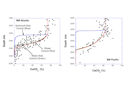
In a recent study published in Geochimica et Cosmochimica Acta, authors have reconciled these divergent experimental results through an equation for the mass balance of the carbonate ion at the sediment-water interface (SWI), which equates the rate of production of that ion via dissolution and its diffusion in sediment porewaters to the transport across the diffusive sublayer (DBL) at the SWI. If the rate constant derived from suspended-grain experiments is inserted into this balance equation, the rate of carbonate ion supply to the SWI from the sediment (sediment-side control) is much greater in the oceans than the rate of transfer across the DBL (water-side control). Thus, calcite dissolution at the seafloor, while technically under mixed control, is strongly water-side dominated. Consequently, a model that neglects boundary-layer transport (sediment-side control alone) invariably predicts CaCO3-versus-depth profiles that are too shallow compared to available data (Figure 1). These new findings will inform future attempts to model the ocean’s response to acidification.
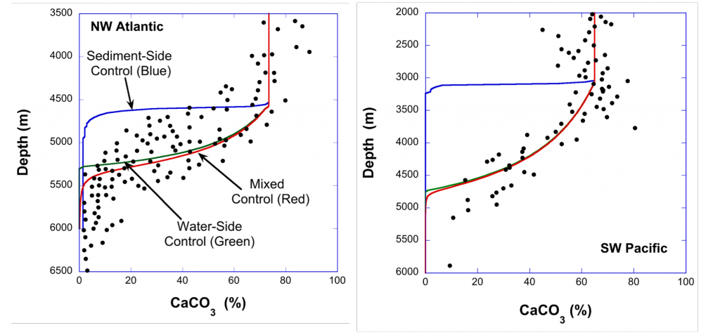
Figure 1: Plots of the calcite (CaCO3) content of deep-sea sediments as a function of oceanic depth. Left panel: data from the Northwestern Atlantic Ocean. Right panel: data from the Southwest Pacific Ocean. The blue line represents predicted CaCO3 content assuming no boundary-layer effects (pure sediment-side control). The red line is the prediction that includes both sediment and water effects (mixed control), and the green line is the prediction with pure water-side control. The agreement between the red and green lines signifies that calcite dissolution is essentially water-side controlled at the seafloor. These results are duplicated for all tested regions of the oceans.
Authors:
Bernard P. Boudreau (Dalhousie University)
Olivier Sulpis (University of Utrecht)
Alfonso Mucci (McGill University)