Ocean Carbon & Biogeochemistry
Studying marine ecosystems and biogeochemical cycles in the face of environmental change
  • Home
  • About OCB
    • About Us
    • Scientific Breadth
      • Biological Pump
      • Changing Marine Ecosystems
      • Changing Ocean Chemistry
      • Estuarine and Coastal Carbon Fluxes
      • Ocean Carbon Uptake and Storage
      • Ocean Observatories
    • Code of Conduct
    • Get Involved
    • Project Office
    • Scientific Steering Committee
    • OCB committees
      • Ocean Time-series
      • US Biogeochemical-Argo
      • Ocean-Atmosphere Interaction
  • Activities
    • Summer Workshop
    • OCB Webinars
    • Guidelines for OCB Workshops & Activities
    • Topical Workshops
      • CMIP6 Models Workshop
      • Coastal BGS Obs with Fisheries
      • C-saw extreme events workshop
      • Expansion of BGC-Argo and Profiling Floats
      • Fish, fisheries and carbon
      • Future BioGeoSCAPES program
      • GO-BCG Scoping Workshop
      • Lateral Carbon Flux in Tidal Wetlands
      • Leaky Deltas Workshop – Spring 2025
      • Marine CDR Workshop
      • Ocean Nucleic Acids ‘Omics
      • Pathways Connecting Climate Changes to the Deep Ocean
    • Small Group Activities
      • Aquatic Continuum OCB-NACP Focus Group
      • Arctic-COLORS Data Synthesis
      • BECS Benthic Ecosystem and Carbon Synthesis WG
      • Carbon Isotopes in the Ocean Workshop
      • CMIP6 WG
      • Filling the gaps air–sea carbon fluxes WG
      • Fish Carbon WG
      • Meta-eukomics WG
      • mCDR
      • Metaproteomic Intercomparison
      • Mixotrophs & Mixotrophy WG
      • N-Fixation WG
      • Ocean Carbonate System Intercomparison Forum
      • Ocean Carbon Uptake WG
      • OOI BGC sensor WG
      • Operational Phytoplankton Observations WG
      • Phytoplankton Taxonomy WG
    • Other Workshops
    • Science Planning
      • Coastal CARbon Synthesis (CCARS)
      • North Atlantic-Arctic
    • Ocean Acidification PI Meetings
    • Training Activities
      • PACE Hackweek 2025
      • PACE Hackweek 2024
      • PACE Training Activity 2022
  • Science Support
    • Data management and archival
    • Early Career
    • Funding Sources
    • Jobs & Postdocs
    • Meeting List
    • OCB Topical Websites
      • Ocean Fertilization
      • Trace gases
      • US IIOE-2
    • Outreach & Education
    • Promoting your science
    • Student Opportunities
    • OCB Activity Proposal Solicitations
      • Guidelines for OCB Workshops & Activities
    • Travel Support
  • Publications
    • OCB Workshop Reports
    • Science Planning and Policy
    • Newsletter Archive
  • Science Highlights
  • News

Archive for scale

Estimating the large-scale biological pump: Do eddies matter?

Posted by mmaheigan 
· Wednesday, December 4th, 2019 

One factor that limits our capacity to quantify the ocean biological carbon pump is uncertainty associated with the physical injection of particulate (POC) and dissolved (DOC) organic carbon to the ocean interior. It is challenging to integrate the effects of these pumps, which operate at small spatial (<100 km) and temporal (<1 month) scales. Previous observational and fine-scale modeling studies have thus far been unable to quantify these small-scale effects. In a recent study published in Global Biogeochemical Cycles, authors explored the influence of these physical carbon pumps relative to sinking (gravity-driven) particles on annual and regional scales using a high-resolution (2 km) biophysical model of the North Atlantic that simulates intense eddy-driven subduction hotspots that are consistent with observations.

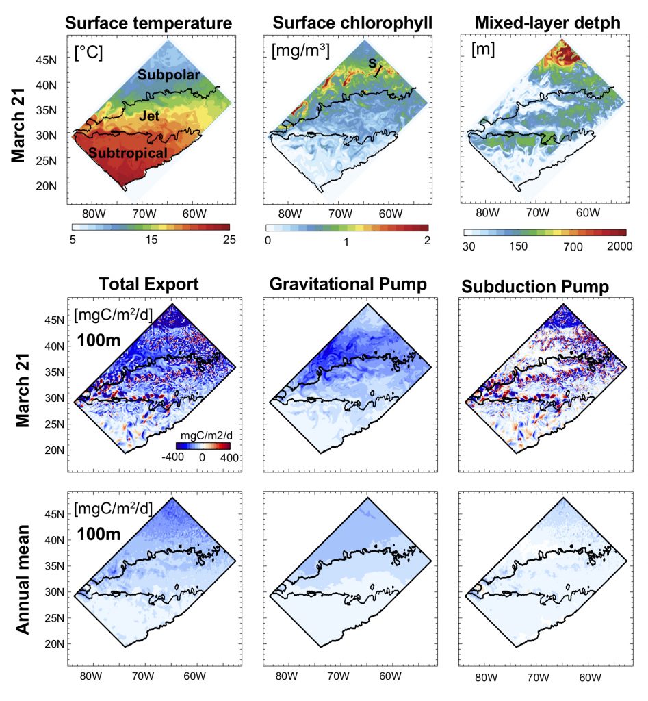
Figure 1: North Atlantic idealized double gyre ocean biophysical model. Top: Sea surface temperature, surface chlorophyll and mixed-layer depth during the spring bloom (March 21). Bottom: total export of organic carbon (POC+DOC) at 100 and individual contributions from the gravitational (particle sinking) and subduction (mixing, eddy advection and Ekman pumping) pumps for one day during the spring bloom (March 21) and averaged annually. Physical subduction hotspots visible on the daily export contribute little to the annual export due to strong compensation of upward and downward motions.

The authors showed that eddy dynamics can transport carbon below the mixed-layer (500-1000 m depth), but this mechanism contributes little (<5%) to annual export at the basin scale due to strong compensation between upward and downward fluxes (Figure 1). Additionally, the authors evidenced that small-scale mixing events intermittently export large amounts of suspended DOC and POC.

These results underscore the need to expand the traditional view of the mixed-layer carbon pump (wintertime export of DOC) to include downward mixing of POC associated with short-lived springtime mixing events, as well as eddy-driven subduction, which can contribute to longer-term ocean carbon storage. High-resolution measurements are needed to validate these model results and constrain the magnitude of the compensation between upward and downward carbon transport by small-scale physical processes.


Authors:
Laure Resplandy (Princeton University)
Marina Lévy (Sorbonne Université)
Dennis J. McGillicuddy Jr. (WHOI)

A framework for ENSO predictability of marine ecosystem drivers along the US West Coast

Posted by mmaheigan 
· Thursday, February 16th, 2017 

The US West Coast eastern boundary upwelling system supports one of the most productive marine ecosystems in the world and is a primary source of ecosystem services for the US (e.g., fishing, shipping, and recreation). Long-term historical observations of physical and biological variables in this region have been collected since the 1950s (e.g., the CalCOFI program and now including the coastal ocean observing systems), leading to an excellent foundation for understanding the ecosystem impacts of dominant climate fluctuations such as the El Niño-Southern Oscillation (ENSO). In the northeast Pacific, ENSO impacts a wide range of physical and biotic processes, including temperature, stratification, winds, upwelling, and primary and secondary production. The El Niño phase of ENSO, in particular, can result in extensive geographic habitat range displacements and altered catches of fishes and invertebrates, and impact vertical and lateral export fluxes of carbon and other elements (Jacox et al., this issue; Anderson et al., this issue; Ohman et al., this issue). However, despite empirical observations and increased understanding of the coupling between climate and marine ecosystems along the US West Coast, there has been no systematic attempt to use this knowledge to forecast marine ecosystem responses to individual ENSO events. ENSO forecasting has become routine in the climate community. However, little has been done to forecast the impacts of ENSO on ecosystems and their services. This becomes especially important considering the occurrence of recent strong El Niño events (such as 2015-16) and climate model projections that suggest that ENSO extremes may become more frequent (Cai et al. 2015).

The joint US CLIVAR/OCB/NOAA/PICES/ICES workshop on Forecasting ENSO impacts on marine ecosystems of the US West Coast (Di Lorenzo et al. 2017) held in La Jolla, California, in August 2016 outlined a three-step strategy to better understand and quantify the ENSO-related predictability of marine ecosystem drivers along the US West Coast (Figure 1). The first step is to use a high-resolution ocean reanalysis to determine the association between local ecosystem drivers and regional forcing patterns (RFPs). The identification of ecosystem drivers will depend on the ecosystem indicators or target species selected for prediction (Ohman et al., this issue). The second step is to objectively identify the tropical sea surface temperature (SST) patterns that optimally force the RFPs along the US West Coast region using available long-term large-scale reanalysis products. While the goal of the first two steps is to understand the dynamical basis for predictability (Figure 1, blue path), the final third step (Figure 1, orange path) aims at quantifying the predictability of the RFPs and estimating their prediction skill at seasonal timescales. This third step can be implemented using the output of multi-model ensemble forecasts such as the North America Multi-Model Ensemble (NMME) or by building efficient statistical prediction models such as Linear Inverse Models (LIMs; Newman et al. 2003).

Figure 1. Framework for understanding and predicting ENSO impacts on ecosystem drivers. Blue path shows the steps that will lead to Understanding of the ecosystem drivers and their dependence on tropical Pacific anomalies. Orange path shows the steps that will lead to quantifying the Predictability of marine ecosystem drivers along the US West Coast that are predictable from large-scale tropical teleconnection dynamics.


Important to the concept of ENSO predictability is the realization that the expressions of ENSO are very diverse and cannot be identified with a few indices (Capotondi et al. 2015; Capotondi et al., this issue). In fact, different expressions of sea surface temperature anomalies (SSTa) in the tropics give rise to oceanic and atmospheric teleconnections that generate different coastal impacts in the northeast Pacific. For this reason, we will refer to ENSO as the collection of tropical Pacific SSTa that lead to deterministic and predictable responses in the regional ocean and atmosphere along the US West Coast.

In the sections below, we articulate in more detail the elements of the framework for quantifying the predictability of ENSO-related impacts on coastal ecosystems along the US West Coast (Figure 1). Our focus will be on the California Current System (CCS), reflecting the regional expertise of the workshop participants. Specifically, we discuss (1) the ecosystem drivers and what is identified as such; (2) RFP definitions; and (3) the teleconnections from the tropical Pacific and their predictability.

Ecosystem drivers in the California Current System

The impacts of oceanic processes on the CCS marine ecosystem have been investigated since the 1950s when the long-term California Cooperative Oceanic Fisheries Investigations (CalCOFI) began routine seasonal sampling of coastal ocean waters. The CalCOFI program continues today and has been augmented with several other sampling programs (e.g., the coastal ocean observing network), leading to an unprecedented understanding of how climate and physical ocean processes, such as upwelling, drive ecosystem variability and change (e.g., see more recent reviews from King et al.2011; Ohman et al. 2013; Di Lorenzo et al. 2013).

The dominant physical oceanographic drivers of ecosystem variability occur on seasonal, interannual, and decadal timescales and are associated with changes in (1) SST; (2) upwelling velocity; (3) alongshore transport; (4) cross-shore transport; and (5) thermocline/nutricline depth (see Ohman et al., this issue). This set of ecosystem drivers emerged from discussions among experts at the workshop. Ecosystem responses to these drivers include multiple trophic levels, including phytoplankton, zooplankton, small pelagic fish, and top predators, and several examples have been identified for the CCS (see summary table in Ohman et al., this issue).

While much research has focused on diagnosing the mechanisms by which these physical drivers impact marine ecosystems, less is known about the dynamics controlling the predictability of these drivers. As highlighted in Ohman et al. (this issue), most of the regional oceanographic drivers (e.g., changes in local SST, upwelling, transport, thermocline depth) are connected to changes in large-scale forcings (e.g., winds, surface heat fluxes, large-scale SST and sea surface height patterns, freshwater fluxes, and remotely forced coastally trapped waves entering the CCS from the south). In fact, several studies have documented how large-scale changes in wind patterns associated with the Aleutian Low and the North Pacific Oscillation drive oceanic modes of variability such as the Pacific Decadal Oscillation and the North Pacific Gyre Oscillation (Mantua et al. 1997; Di Lorenzo et al. 2008; Chhak et al. 2009; Ohman et al., this issue; Jacox et al., this issue; Anderson et al., this issue; Capotondi et al., this issue) that influence the CCS. However, these large-scale modes only explain a fraction of the ecosystem’s atmospheric forcing functions at the regional-scale. Thus, it is important to identify other key forcings to gain a more complete mechanistic understanding of CCS ecosystem drivers (e.g., Jacox et al. 2014; 2015).

Atmospheric and oceanic regional forcing patterns

The dominant large-scale quantities that control the CCS ecosystem drivers are winds, heat fluxes, and remotely forced coastally trapped waves (Hickey 1979). Regional expressions or patterns of these large-scale forcings have been linked to changes in local stratification and thermocline depth (Veneziani et al. 2009a; 2009b; Combes et al. 2013), cross-shore transport associated with mesoscale eddies (Kurian et al. 2011; Todd et al. 2012; Song et al. 2012; Davis and Di Lorenzo 2015b), and along-shore transport (Davis and Di Lorenzo 2015a; Bograd et al. 2015). For this reason, we define the regional expressions of the atmospheric and remote wave forcing that are optimal in driving SST, ocean transport, upwelling, and thermocline depth as the RFPs. To clarify this concept, consider the estimation of coastal upwelling velocities. While a change in the position and strength in the Aleutian Low has been related to coastal upwelling in the northern CCS, a more targeted measure of the actual upwelling vertical velocity and nutrient fluxes that are relevant to primary productivity can only be quantified by taking into account a combination of oceanic processes that depend on multiple RFPs such as thermocline depth (e.g., remote waves), thermal stratification (e.g., heat fluxes), mesoscale eddies, and upwelling velocities (e.g., local patterns of wind stress curl and alongshore winds; see Gruber et al 2011; Jacox et al. 2015; Renault et al. 2016). In other words, if we consider the vertical coastal upwelling velocity (w) along the northern CCS, a more adequate physical description and quantification would be given from a linear combination of the different regional forcing functions w = Σn ∝n * RFPn rather than w = ∝*Aleutian Low.

The largest interannual variability in the Pacific that impacts the RFPs is ENSO, which also constitutes the largest source of seasonal (3-6 months) predictability. During El Niño and La Niña, atmospheric and oceanic teleconnections from the tropics modify large-scale and local surface wind patterns and ocean currents of the CCS and force coastally trapped waves.

ENSO teleconnections and potential seasonal predictability of the regional forcing patterns

While ENSO exerts important controls on the RFPs in the CCS, it has become evident that ENSO expressions in the tropics vary significantly from event to event, leading to different responses in the CCS (Capotondi et al., this issue). Also, as previously pointed out, the CCS is not only sensitive to strong ENSO events but more generally responds to a wide range of tropical SSTa variability that is driven by ENSO-type dynamics in the tropical and sub-tropical Pacific. For this reason, we define an “ENSO teleconnection” as any RFP response that is linked to ENSO-type variability in the tropics.

ENSO can influence the upwelling and circulation in the CCS region through both oceanic and atmospheric pathways. It is well known that equatorial Kelvin waves, an integral part of ENSO dynamics, propagate eastward along the Equator and continue both northward (and southward) along the coasts of the Americas as coastally trapped Kelvin waves after reaching the eastern ocean boundary. El Niño events are associated with downwelling Kelvin waves, leading to a deepening of the thermocline, while La Niña events produce a shoaling of the thermocline in the CCS (Simpson 1984; Lynn and Bograd 2002; Huyer et al. 2002; Bograd et al. 2009; Hermann et al. 2009; Miller et al. 2015). The offshore scale of coastal Kelvin waves decreases with latitude, and the waves decay while propagating northward along the coast due to dissipation and radiation of westward propagating Rossby waves. In addition, topography and bathymetry can modify the nature of the waves and perhaps partially impede their propagation at some location. Thus, the efficiency of coastal waves of equatorial origin in modifying the stratification in the CCS is still a matter of debate. To complicate matters, regional wind variability south of the CCS also excites coastally trapped waves, which supplement the tropical source.

In the tropics, SST anomalies associated with ENSO change tropical convection and excite mid-troposphere stationary atmospheric Rossby waves that propagate signals to the extratropics, the so-called atmospheric ENSO teleconnections (Capotondi et al., this issue). Through these atmospheric waves, warm ENSO events favor a deepening and southward shift of the Aleutian Low pressure system that is dominant during winter, as well as changes in the North Pacific Subtropical High that is dominant during spring and summer, resulting in a weakening of the alongshore winds, reduced upwelling, and warmer surface water. These changes are similar to those induced by coastal Kelvin waves of equatorial origin, making it very difficult to distinguish the relative importance of the oceanic and atmospheric pathways in the CCS. In addition, due to internal atmospheric noise, the details of the ENSO teleconnections can vary significantly from event to event and result in important differences along the California Coast (Figure 2).

Figure 2. Schematic of ENSO teleconnection associated with different flavors of tropical SSTa. (a) Atmospheric teleconnections of the canonical eastern Pacific El Niño tend to impact the winter expression of the Aleutian Low, which in turn drives an oceanic SSTa anomaly that projects onto the pattern of the Pacific Decadal Oscillation (PDO). (b) Atmospheric teleconnections of the central Pacific El Niño tend to impact the winter expression of the North Pacific High, which in turn drives an oceanic SSTa anomaly that projects onto the pattern of the North Pacific Gyre Oscillation (NPGO). The ENSO SSTa maps are obtained by regressing indices of central and eastern Pacific ENSO with SSTa. The other maps are obtained by regression of SSTa/SLPa with the PDO (a) and NPGO (b) indices.


El Niño events exhibit a large diversity in amplitude, duration, and spatial pattern (Capotondi et al. 2015). The amplitude and location of the maximum SST anomalies, whether in the eastern (EP) or central (CP) Pacific, can have a large impact on ENSO teleconnections (Ashok et al. 2007; Larkin and Harrison 2005). While “canonical” EP events induce changes in the Aleutian Low (Figure 2b), CP events have been associated with a strengthening of the second mode of North Pacific atmospheric variability, the North Pacific Oscillation (NPO; Figure 2a; Di Lorenzo et al. 2010; Furtado et al. 2012). In addition, it is conceivable that EP events have a larger Kelvin wave signature than CP events, resulting in different oceanic influences in the CCS.

In summary, while the ENSO influence on the CCS physical and biological environments is undeniable, several sources of uncertainty remain about the details of that influence. This uncertainty arises in the physical environment on seasonal timescales from many sources, including the diversity of ENSO events, the intrinsic unpredictable components of the atmosphere, and the intrinsic unpredictable eddy variations in the CCS. We also need to distinguish between physically forced ecosystem response versus intrinsic biological variability, which is potentially nonlinear and likely unpredictable. Skill levels need to be quantified for each step of the prediction process (i.e., ENSO, teleconnections, local oceanic response, local ecosystem response) relative to a baseline—for example the persistence of initial condition, which is also being exploited for skillful predictions of the large marine ecosystem at the seasonal timescale (Tommasi et al., this issue). The target populations should be exploitable species that are of interest to federal and state agencies that regulate certain stocks. Models are currently being developed to use ocean forecasts to advance top predator management (Hazen et al., this issue). The implementation of this framework (Figure 1) for practical uses will require a collaborative effort between physical climate scientists with expertise in predicting and understanding ENSO and biologists who have expertise in understanding ecosystem response to physical climate forcing.

Authors

Emanuele Di Lorenzo (Georgia Institute of Technology)
Arthur J. Miller (Scripps Institution of Oceanography)

References

Ashok, K., S.K. Behera, S.A. Rao, H. Weng, and T. Yamagata, 2007: El Niño Modoki and its possible teleconnections. J. Geophys. Res., 112, doi:10.1029/2006JC003798

Bograd, S. J., M. Pozo Buil, E. Di Lorenzo, C. G. Castro, I. D. Schroeder, R. Goericke, C. R. Anderson, C. Benitez-Nelson, and F. A. Whitney, 2015: Changes in source waters to the Southern California Bight. Deep-Sea Res. Part II-Top. Stud. Oceanogr., 112, 42-52, doi:10.1016/j.dsr2.2014.04.009.

Bograd, S. J., I. Schroeder, N. Sarkar, X. Qiu, W. J. Sydeman, and F. B. Schwing, 2009: Phenology of coastal upwelling in the California Current. Geophy. Res. Lett., 36, doi: 10.1029/2008GL035933.

Cai, W. J., and Coauthors, 2015: ENSO and greenhouse warming. Nature Climate Change, 5, 849-859, doi:10.1038/nclimate2743.

Capotondi, A., and Coauthors, 2015: Understanding ENSO Diversity. Bull. Amer. Meteor. Soc., 96, 921-938, doi:10.1175/BAMS-D-13-00117.1.

Chhak, K. C., E. Di Lorenzo, N. Schneider, and P. F. Cummins, 2009: Forcing of low-frequency ocean variability in the northeast Pacific. J. Climate, 22, 1255-1276, doi:10.1175/2008jcli2639.1.

Davis, A., and E. Di Lorenzo, 2015a: Interannual forcing mechanisms of California Current transports I: Meridional Currents. Deep-Sea Res. Part II-Top. Stud. Oceanogr., 112, 18-30, doi:10.1016/j.dsr2.2014.02.005.

Davis, A., and E. Di Lorenzo, 2015b: Interannual forcing mechanisms of California Current transports II: Mesoscale eddies. Deep-Sea Res. Part II-Top. Stud. Oceanogr., 112,  31-41, doi:10.1016/j.dsr2.2014.02.004.

Di Lorenzo, E., and Coauthors, 2017: Forecasting ENSO impacts on marine ecosystems of the US West Coast, Joint US CLIVAR/NOAA/PICES/ICES Report, https://usclivar.org/meetings/2016-enso-ecosystems, forthcoming.

Di Lorenzo, E., and Coauthors, 2008: North Pacific Gyre Oscillation links ocean climate and ecosystem change. Geophys. Res. Lett., 35, doi:10.1029/2007gl032838.

Di Lorenzo, E., and Coauthors, 2013: Synthesis of Pacific Ocean climate and ecosystem dynamics. Oceanogr., 26, 68-81, doi: 10.5670/oceanog.2013.76.

Di Lorenzo, E., K. M. Cobb, J. C. Furtado, N. Schneider, B. T. Anderson, A. Bracco, M. A. Alexander, and D. J. Vimont, 2010: Central Pacific El Nino and decadal climate change in the North Pacific Ocean. Nature Geosci., 3, 762-765, doi:10.1038/ngeo984.

Furtado, J. C., E. Di Lorenzo, B. T. Anderson, and N. Schneider, 2012: Linkages between the North Pacific Oscillation and central tropical Pacific SSTs at low frequencies. Climate Dyn., 39, 2833-2846, doi:10.1007/s00382-011-1245-4.

Gruber, N., Z. Lachkar, H. Frenzel, P. Marchesiello, M. Munnich, J. C. McWilliams, T. Nagai, and G. K. Plattner, 2011: Eddy-induced reduction of biological production in eastern boundary upwelling systems. Nature Geosci., 4, 787-792, doi:10.1038/ngeo1273.

Hermann, A. J., E. N. Curchitser, D. B. Haidvogel, and E. L. Dobbins, 2009: A comparison of remote vs. local influence of El Nino on the coastal circulation of the northeast Pacific. Deep Sea Res. Part II: Top. Stud. Oceanogr., 56, 2427-2443, doi: 10.1016/j.dsr2.2009.02.005.

Hickey, B. M., 1979. The California Current system—hypotheses and facts. Prog. Oceanogr., 8, 191-279, doi: 10.1016/0079-6611(79)90002-8.

Huyer, A., R. L. Smith, and J. Fleischbein, 2002: The coastal ocean off Oregon and northern California during the 1997–8 El Nino. Prog. Oceanogr., 54, 311-341, doi: 10.1016/S0079-6611(02)00056-3.

Jacox, M. G., A. M. Moore, C. A. Edwards, and J. Fiechter, 2014: Spatially resolved upwelling in the California Current System and its connections to climate variability. Geophy. Res. Lett., 41, 3189-3196, doi:10.1002/2014gl059589.

Jacox, M. G., J. Fiechter, A. M. Moore, and C. A. Edwards, 2015: ENSO and the California Current coastal upwelling response. J. Geophy. Res.-Oceans, 120, 1691-1702, doi:10.1002/2014jc010650.

Jacox, M. G., S. J. Bograd, E. L. Hazen, and J. Fiechter, 2015: Sensitivity of the California Current nutrient supply to wind, heat, and remote ocean forcing. Geophys. Res. Lett., 42, 5950-5957, doi:10.1002/2015GL065147.

Jacox, M. G., E. L. Hazen, K. D. Zaba, D. L. Rudnick, C. A. Edwards, A. M. Moore, and S. J. Bograd, 2016: Impacts of the 2015-2016 El Niño on the California Current System: Early assessment and comparison to past events. Geophys. Res. Lett., 43, 7072-7080, doi:10.1002/2016GL069716.

King, J. R., V. N. Agostini, C. J. Harvey, G. A. McFarlane, M. G. G. Foreman, J. E. Overland, E. Di Lorenzo, N. A. Bond, and K. Y. Aydin, 2011: Climate forcing and the California Current ecosystem. Ices J. Mar. Sci., 68, 1199-1216, doi:10.1093/icesjms/fsr009.

Kurian, J., F. Colas, X. Capet, J. C. McWilliams, and D. B. Chelton, 2011: Eddy properties in the California Current System. J. Geophy. Res.-Oceans, 116, doi:10.1029/2010jc006895.

Larkin, N. K. and D. E. Harrison, 2005: On the definition of El Niño and associated seasonal average US weather anomalies. Geophy. Res. Lett. 32, doi: 10.1029/2005GL022738.

Lynn, R. J. and S. J. Bograd, 2002: Dynamic evolution of the 1997–1999 El Niño–La Niña cycle in the southern California Current system. Prog. Oceanogr., 54, 59-75, doi: 10.1016/S0079-6611(02)00043-5.

Mantua, N. J., S. R. Hare, Y. Zhang, J. M. Wallace, and R. C. Francis, 1997: A Pacific interdecadal climate oscillation with impacts on salmon production. Bull. Amer. Meteorol. Soc., 78, 1069-1079, doi:10.1175/1520-0477(1997)078<1069:apicow>2.0.co;2.

Marchesiello, P., J. C. McWilliams, and A. Shchepetkin, 2003: Equilibrium structure and dynamics of the California Current System. J. Phys. Oceanogr., 33, 753-783, doi: 10.1175/1520-0485(2003)33<753:ESADOT>2.0.CO;2.

McCreary, J. P., P. K. Kundu, and S. Y. Chao, 1987: On the dynamics of the California Current System. J. Mar. Res., 45, 1-32, doi: 10.1357/002224087788400945.

Miller, A. J., H. Song, and A. C. Subramanian, 2015: The physical oceanographic environment during the CCE-LTER Years: Changes in climate and concepts. Deep Sea Res. Part II: Top. Stud. Oceanogr., 112, 6-17, doi: 10.1016/j.dsr2.2014.01.003.

Newman, M., and Coauthors, 2016: The Pacific Decadal Oscillation, Revisited. J. Climate, 29, 4399-4427, doi:10.1175/jcli-d-15-0508.1.

Ohman, M. D., K. Barbeau, P. J. S. Franks, R. Goericke, M. R. Landry, and A. J. Miller, 2013: Ecological transitions in a coastal upwelling ecosystem. Oceanogr., 26, 210-219, doi: 10.5670/oceanog.2013.65.

Renault, L., C. Deutsch, J. C. McWilliams, H. Frenzel, J.-H. Liang, and F. Colas, 2016: Partial decoupling of primary productivity from upwelling in the California Current system. Nature Geosci, 9, 505-508, doi:10.1038/ngeo2722.

Simpson, J. J., 1984; El Nino‐induced onshore transport in the California Current during 1982‐1983. Geophy. Res. Lett., 11, 233-236, doi: 10.1029/GL011i003p00233.

Song, H., A. J. Miller, B. D. Cornuelle, and E. Di Lorenzo, 2011: Changes in upwelling and its water sources in the California Current System driven by different wind forcing. Dyn. Atmos. Oceans, 52, 170-191, doi:10.1016/j.dynatmoce.2011.03.001.

Todd, R. E., D. L. Rudnick, M. R. Mazloff, B. D. Cornuelle, and R. E. Davis, 2012: Thermohaline structure in the California Current System: Observations and modeling of spice variance. J. Geophy. Res.-Oceans, 117, doi:10.1029/2011jc007589.

Veneziani, M., C. A. Edwards, J. D. Doyle, and D. Foley, 2009: A central California coastal ocean modeling study: 1. Forward model and the influence of realistic versus climatological forcing. J. Geophy. Res.-Oceans, 114, doi:10.1029/2008jc004774.

Veneziani, M., C. A. Edwards, and A. M. Moore, 2009: A central California coastal ocean modeling study: 2. Adjoint sensitivities to local and remote forcing mechanisms. J. Geophy. Res.-Oceans, 114, doi:10.1029/2008jc004775.


ENSO diversity and its implications for US West Coast marine ecosystems

Posted by mmaheigan 
· Thursday, February 16th, 2017 

The El Niño-Southern Oscillation (ENSO) is the dominant mode of tropical Pacific climate variability at interannual timescales, with profound influences on seasonal weather and ecosystems worldwide. In particular, the physical and biological conditions along the US West Coast, an area that supports one of the most productive marine ecosystems in the world, are strongly influenced by ENSO. Specifically, during El Niño events, alongshore winds weaken and upwelling is reduced, resulting in warmer surface waters, reduced nutrient supply to the euphotic zone, and reduced biological productivity. While these conditions during El Niño events are well known, the exact mechanisms involved and the origin of event-to-event differences in ENSO impacts are not fully understood. Here, we review our current state of knowledge on ENSO and its different expressions, the mechanisms by which ENSO influences the US West Coast, and possible approaches for understanding the predictability of those impacts.

ENSO dynamics and oceanic teleconnections

Tropical Pacific interannual variations involve changes in the thermocline, namely the interface between the warmer upper ocean layer and the colder deeper ocean. In its neutral state, the tropical Pacific is characterized by a shallower thermocline in the eastern Pacific and deeper thermocline in the western Pacific, with a zonal (east-west) slope that is in equilibrium with the surface easterly wind stress. Surface waters are thus colder in the eastern Pacific “Cold Tongue,” and much warmer west of the dateline in the western Pacific “Warm Pool.” ENSO events are disruptions of this neutral state. During warm events, the El Niño phase, the easterly trades weaken, reducing upwelling in the Cold Tongue region. The thermocline deepens in the east and shoals in the west (Figure 1) and the zonal temperature gradient is reduced. The initial deepening of the eastern Pacific thermocline is achieved through the eastward propagation of downwelling Kelvin waves, excited by high-frequency winds in the form of westerly wind events (WWEs) in the western Pacific (McPhaden 1999, Roundy and Kiladis 2006), and amplified by slower-building wind anomalies (known as the Bjerknes feedback). After reaching the eastern ocean boundary, these Kelvin waves continue poleward along the coastlines of the Americas as coastally trapped Kelvin waves, depressing the thermocline, and reducing upwelling along the west coast of North and South America. The coastal wave propagation north of the Equator can clearly be seen in Figure 1 all the way to Baja California. In contrast, upwelling Kelvin waves during La Niña conditions induce a shoaling of the thermocline in the eastern equatorial Pacific and along the west coast of the Americas, resulting in increased upwelling (Simpson 1984; Lynn and Bograd 2002; Huyer et al. 2002; Bograd et al. 2009; Hermann et al. 2009; Miller et al. 2015).

Figure 1. Canonical oceanic teleconnection pattern associated with coastally trapped Kelvin waves emanating from the tropical and subtropical eastern Pacific during the 1997-98 El Niño, as revealed by sea surface height altimeter observations (Credit: NASA/JPL-Caltech). These boundary-trapped waves have the potential to travel from the Equatorial region to the California Coast (and beyond) where they can alter thermocline depth, SST, mixed-layer depth, and currents. Atmospheric teleconnections, however, can also drive regional oceanic anomalies that mimic this same type of response.


The changes in upwelling associated with the coastal Kelvin waves can directly impact the biogeochemistry of the waters along the US West Coast. However, the offshore scale of the waves decreases with latitude, and the waves decay while propagating northward due to dissipation and radiation of energy by the generation of westward propagating Rossby waves (Marchesiello et al. 2003). In addition, topography and bathymetry can modify the nature of the waves and perhaps partially impede their propagation at some locations, casting some doubt on the effectiveness of coastal waves of equatorial origin to substantially alter the stratification along the US West Coast and modulate the local marine ecosystem.

Atmospheric teleconnections

Equatorial sea surface temperature (SST) anomalies associated with ENSO also influence remote weather and climate through large-scale atmospheric teleconnections. Variations in convection trigger atmospheric stationary Rossby wave trains that alter the Pacific North America Pattern (PNA, Figure 2), a mode of North Pacific geopotential height variability (Horel and Wallace 1981), and induce variations in the regional atmospheric circulation. In particular, El Niño events are associated with an intensification and southward shift of the Aleutian Low (AL) pressure system and changes in the eastern Pacific subtropical high, which conspire to weaken the alongshore winds off the US West Coast, resulting in reduced upwelling and warmer SST. These changes associated with the local atmospheric forcing are similar to those induced by coastal Kelvin waves of equatorial origin, making it very difficult to distinguish the relative importance of the oceanic and atmospheric pathways in this region, especially observationally. In addition, large uncertainties exist surrounding the atmospheric mid-latitude response to tropical SST anomalies. Results from a recent study based on both observations and climate model ensemble simulations indicate that uncertainties in the sea level pressure (SLP) response to ENSO arise primarily from atmospheric internal variability rather than diversity in ENSO events (Deser et al. 2017). Thus, the details of the ENSO teleconnections can vary significantly and randomly from event to event and result in important differences along the California Coast.

Figure 2. Canonical wintertime atmospheric teleconnection pattern associated with ENSO as a response to tropical heating, also known as the Pacific North American (PNA) pattern, as schematically illustrated by Horel and Wallace (1981). The contour lines represent middle troposphere geopotential height anomalies that occur in response to warm SST in the tropical Pacific near the dateline during an El Niño (shaded area). The Rossby wave-like pattern includes high-pressure anomalies in the Northern Hemispheric subtropics and low-pressure anomalies in the North Pacific, with a ridge over Canada and an anomalous low-pressure region in the Southeastern US. The dark arrows depict the strengthened subtropical jets and easterlies near the dateline. The lighter arrows indicate the distorted mid-tropospheric streamlines due to troughing and ridging.


ENSO diversity and its implications for impacts on the US West Coast

As already noted by Wyrtki (1975), “No two El Niño events are quite alike.” Indeed, ENSO events differ in amplitude, duration, and spatial pattern, and several studies have suggested that such differences may play an important role in ENSO impacts (see Capotondi et al. 2015 for a review). Special emphasis has been given to the location of the maximum equatorial SST anomalies, as this is an aspect that is readily observed and may influence atmospheric teleconnections (Ashok et al. 2007; Larkin and Harrison 2005). Although the longitudinal position of the maximum SST anomalies along the equator varies from event to event in a quasi-continuum fashion, for practical purposes, events are often grouped depending on whether the largest anomalies are located in the eastern Pacific (“EP” events), or in the central Pacific (“CP” events). Here, we use the relative amplitudes of SST anomalies in the Niño-3 (5°S-5°N, 150°W-90°W) and Niño-4 (5°S-5°N, 160°E-150°W) regions to classify the events as “EP” or “CP”. Figure 3 shows the equatorial profiles of SST anomalies for the two groups of events in the Simple Ocean Data Assimilation (SODA; Carton and Giese 2008) reanalysis over the period 1958-2007 (Figure 3a) and in 500 years of a pre-industrial control simulation of the National Center for Atmospheric Research (NCAR) Community Climate System Model version 4 (CCSM4; Figure 3b). We notice that there is a large overlap between the two groups of events, which is indicative of the large spread in event longitudinal distribution, although events peaking in the eastern Pacific can achieve larger amplitudes than those peaking in the central Pacific. This difference in amplitude is not as pronounced in the precipitation profiles (Figure 3c), suggesting that in spite of their weaker SST anomaly signature, CP events may still have a large influence on the atmosphere due to their position in a region of warmer background SST.

Figure 3. a) Equatorial SST anomaly profiles for El Niño events with largest SST anomalies in the Niño-3 region (EP events, thin dashed orange lines) and in the Niño-4 region (CP events, thin dashed blue lines) from the SODA ocean reanalysis over the period 1958-2007. The thick red and blue lines are the composites of the thin orange and blue lines, respectively. b) Same as in a, but for a 500-year preindustrial simulation of the NCAR-CCSM4 climate model. c) Same as in b, but for precipitation anomalies rather than SST anomalies. The a), b) and c) panels are adapted from Capotondi (2013). d) Tropical SST anomaly pattern, or “sensitivity pattern,” that exerts the largest influence on the PNA (the “+” and “-“ signs indicate the PNA highs and lows as shown in Figure 2), as computed by Barsugli and Sardeshmukh (2002) using ensembles of atmospheric model simulations forced by a set of SST anomaly patches over the tropical Pacific. Panel c) is adapted from Barsugli and Sardeshmukh (2002).


Do different types of ENSO events have different impacts on the climate and marine ecosystems of the US West Coast? In terms of atmospheric teleconnections, “canonical” EP events have been associated with changes in the AL, while CP events may produce a strengthening of the second mode of North Pacific atmospheric variability, the North Pacific Oscillation (NPO; Di Lorenzo et al. 2013). AL variability is associated with the Pacific Decadal Oscillation, while the NPO appears to provide the atmospheric forcing for the North Pacific Gyre Oscillation (Di Lorenzo et al. 2008), a mode of variability that is largely correlated with biologically relevant quantities along the West Coast of the US. However, the event-to-event differences in teleconnections, associated with intrinsic atmospheric variability, may obscure differences in atmospheric response to different event types.

EP and CP events have different subsurface characteristics as well so that the oceanic pathways between the tropical Pacific and the US West Coast can also be expected to differ in the two cases. While EP events are characterized by large equatorial thermocline anomalies across the basin, which evolve consistently with the recharge oscillator paradigm (Jin 1997), thermocline depth anomalies during CP events tend to be confined to the central part of the basin and do not undergo the large variations associated with the meridional warm water volume transport. As a result, the Kelvin wave signature in the eastern equatorial Pacific, and the resulting amplitude of the coastal Kelvin wave can be expected to be weaker during CP events. Indeed, a recent study (Fischer et al. 2015) has shown that temperature anomalies (and associated zooplankton composition) in the northern California Current responded very rapidly to EP El Niño events with a peak during boreal winter, whereas CP events were accompanied by a delayed response with a peak during boreal spring. The most recent 2015/16 El Niño provides another compelling example of diversity in ENSO influences. In spite of the magnitude of the event, which was comparable to the previous two extreme events on record, the 1982/83 and 1997/98, the changes in temperature, thermocline/nutricline depth, and alongshore winds associated with this event were much smaller than during the two previous cases (Jacox et al. 2016). These differences are perhaps due to the unique nature of this event, whose spatial pattern has elements of both EP and CP El Niño types, with, in particular, a weaker thermocline depth anomaly in the eastern equatorial Pacific relative to the 1982/83 and 1997/98 cases. This question remains open and is the subject of intense research.

How well can we predict different types of ENSO events? Several studies have attempted to determine specific precursors for EP- and CP-type events. SST and wind stress anomalies propagating southwestward from the Southern California coast to the central equatorial Pacific, a pattern known as the “Pacific Meridional Mode” (PMM; Chiang and Vimont 2004) has been suggested as a possible precursor for CP events (Yu and Kim 2011; Vimont et al. 2014), while SST and wind stress anomalies extending northward along the coast of South America toward the eastern equatorial Pacific (the “South Pacific Meridional Mode” or SPMM; Zhang et al. 2014) have been considered as candidate precursors for EP-type events. While these modes of variability do produce initial SST anomalies either in the central or eastern Pacific, these anomalies can propagate along the equator and maximize at a different longitude in the mature phase of the event. For example, the strong 1982/83 EP El Niño developed from anomalous SSTs in the central Pacific in the late spring of 1982, which propagated eastward to achieve their largest amplitude near the South American coast in the following winter (Xue and Kumar 2016). In late spring 2015, on the other hand, anomalies exceeding 2°C appeared in the far eastern Pacific and then propagated westward to reach their largest amplitude in the central Pacific in winter (Xue and Kumar 2016). While several studies have emphasized SST precursors, thermocline conditions two seasons prior to the peak of an event appear to play an important role in the development of the two types of events (Capotondi and Sardeshmukh 2015). Deeper than average initial thermocline conditions in the eastern Pacific favor EP-type events and shallower than average eastern Pacific thermocline depth favors CP-type events. The results of Capotondi and Sardeshmukh (2015) were obtained using a combination of multiple linear regressions and linear inverse modeling (Penland and Sardeshmukh 1995), thus objectively providing the initial state that will optimally evolve, two seasons later, in either an EP- or CP-type event.

Given the remaining uncertainties in the exact triggers of ENSO diversity, as well as the large noise level of atmospheric teleconnections, how can we isolate the predictable component of the ENSO influence on the US West Coast physical and biogeochemical conditions in the Pacific? In other words, even if we could perfectly predict ENSO in all its diversity and atmospheric teleconnections, how well could we predict the ecosystem responses? One possible approach is to determine the SST pattern to which a given target quantity (e.g., a mode of atmospheric variability or some local ecosystem forcing function) is most sensitive. The SST anomalies that are most effective in influencing specific “target” regions do not necessarily coincide with the anomalies typical of “canonical” ENSO events (Rasmussen and Carpenter 1982). In fact, as shown by Barsugli and Sardeshmukh (2002) the PNA pattern is particularly sensitive to SST anomalies in the Niño-4 region rather than the Niño-3 region where canonical “EP” events typically peak (Figure 3d). This implies that weaker CP El Niño events may exert a comparable influence on the sensitivity pattern relative to stronger EP events, and be as (if not more) effective in influencing atmospheric teleconnections like the PNA (compare Figures 3a,b with Figure 3d). Similar sensitivity patterns could be determined for key regional forcing function along the US West Coast, either using the approach outlined in Barsugli and Sardeshmukh (2002) or via multiple linear regression (e.g., Capotondi and Sardeshmukh 2015).

Conclusions

In summary, ENSO can provide a large source of potential predictability for the physics and the biology of the US West Coast. However, in light of the large uncertainties associated with ENSO diversity and atmospheric teleconnections, novel approaches need to be developed to isolate the robust predictable components of ENSO influences and inform forecast development.

Authors

Antonietta Capotondi (NOAA Earth System Research Laboratory)
Kris Karnauskas (University of Colorado, Boulder)
Arthur Miller (Scripps Institution of Oceanography)
Aneesh Subramanian (University of Oxford, UK)

References

Ashok, K., S. K. Behera, S. A. Rao, H. Weng, and T. Yamagata, 2007: El Niño Modoki and its possible teleconnections. J. Geophys. Res., 112, doi:10.1029/2006JC003798.

Barsugli, J. J., and P. D. Sardeshmukh, 2002: Global atmospheric sensitivity to tropical SST anomalies throughout the Indo-Pacific basin. J. Climate, 15, 3427-3442, doi: 10.1175/1520-0442(2002)015<3427:GASTTS>2.0.CO;2.

Bograd, S. J., I. Schroeder, N. Sarkar, X. Qiu, W. J. Sydeman, and F. B. Schwing, 2009: Phenology of coastal upwelling in the California Current. Geophys. Res. Lett., 36, doi: 10.1029/2008GL035933.

Capotondi, A., 2013: ENSO diversity in the NCAR CCSM4 climate model. J. Geophys. Res. Oceans, 118, 4755-4770, doi:10.1002/jgrc.20335.

Capotondi, A., and Coauthors, 2015: Understanding ENSO Diversity. Bull. Amer. Meteor. Soc., 96, 921-938, doi:10.1175/BAMS-D-13-00117.1.

Capotondi, A., and P. D. Sardeshmukh, 2015: Optimal precursors of different types of ENSO events. Geophys. Res. Lett., 42, doi:10.1002/2015GL066171.

Carton, J. A., and B. S. Giese, 2008: A reanalysis of ocean climate using simple ocean data assimilation (SODA). Mon. Wea. Rev., 136, 2999-3017, doi:10.1175/2007MWR1978.1.

Chiang, J. C. H., and D. J. Vimont, 2004: Analogous Pacific and Atlantic meridional modes of tropical atmosphere-ocean variability. J. Climate, 17, 4143-4158, doi: 10.1175/JCLI4953.1.

Deser, C., I. R. Simpson, K. A. McKinnon, and A. S. Phillips, 2017: The Northern Hemisphere extra-tropical atmospheric circulation response to ENSO: How well do we know it and how do we evaluate models accordingly? J. Climate, submitted.

Di Lorenzo, E., and Coauthors, 2008: North Pacific Gyre Oscillation links ocean climate and ecosystem change. Geophys. Res. Lett., 35, doi:10.1029/2007gl032838.

Di Lorenzo, E., and Coauthors, 2013: Synthesis of Pacific Ocean climate and ecosystem dynamics. Oceanogr., 26, 68-81, doi: 10.5670/oceanog.2013.76.

Fischer, J. L., W. T. Peterson, and R. R. Rykaczewski, 2015: The impact of El Niño events on the pelagic food chain in the northern California Current. Glob. Change Bio., 21, 4401-4414, doi:10.1111/gbc.13054.

Hermann, A. J., E. N. Curchitser, D. B. Haidvogel, and E. L. Dobbins, 2009. A comparison of remote vs. local influence of El Nino on the coastal circulation of the northeast Pacific. Deep Sea Res. Part II: Top. Stud. Oceanogr., 56, 2427-2443, doi: 10.1016/j.dsr2.2009.02.005.

Horel, J. D., and J. M. Wallace, 1981: Planetary-scale atmospheric phenomena associated with the Southern Oscillation. Mon. Wea. Rev., 109, 813-829, doi: 10.1175/1520-0493(1981)109<0813:PSAPAW>2.0.CO;2.

Huyer, A., R. L. Smith, and J. Fleischbein, 2002: The coastal ocean off Oregon and northern California during the 1997–8 El Nino. Prog. Oceanogr., 54, 311-341, doi: 10.1016/S0079-6611(02)00056-3.

Jacox, M. G., E. L. Hazen, K. D. Zaba, D. L. Rudnick, C. A. Edwards, A. M. Moore, and S. J. Bograd, 2016: Impacts of the 2015-2016 El Niño on the California Current System: Early assessment and comparison to past events. Geophys. Res. Lett., 43, 7072-7080, doi:10.1002/2016GL069716.

Jin, F.-F., 1997: An equatorial ocean recharge paradigm for ENSO. Part I: Conceptual model. J. Atmos. Sci., 54, 811-829, doi: 10.1175/1520-0469(1997)054<0811:AEORPF>2.0.CO;2.

Larkin, N. K., and D. E., Harrison, 2005: On the definition of El Niño and associated seasonal average U.S. weather anomalies. Geophys. Res. Lett. 32, doi:10.1029/2005GL022738.

Lynn, R. J., and S. J. Bograd,  2002: Dynamic evolution of the 1997–1999 El Niño–La Niña cycle in the southern California Current system. Prog. Oceanogr., 54, 59-75, doi: 10.1016/S0079-6611(02)00043-5..

Marchesiello, P., J. C. McWilliams, and A. Shchepetkin, 2003. Equilibrium structure and dynamics of the California Current System. J. Phys. Oceanogr., 33, 753-783, doi: 10.1175/1520-0485(2003)33<753:ESADOT>2.0.CO;2.

McPhaden, M. J., 1999: Climate oscillations – Genesis and evolution of the 1997-98 El Niño. Science, 283, 950-954.

Miller, A. J., H. Song, and A. C. Subramanian, 2015: The physical oceanographic environment during the CCE-LTER Years: Changes in climate and concepts. Deep Sea Res. Part II: Top. Stud. Oceanogr., 112, 6-17, doi: 10.1016/j.dsr2.2014.01.003.

Penland, C., and P. D. Sardeshmukh, 1995: The optimal growth of tropical sea surface temperature anomalies. J. Climate, 8, 1999-2024, doi: 10.1175/1520-0442(1995)008<1999:TOGOTS>2.0.CO;2.

Rasmusson, E. M., and T. H. Carpenter, 1982: Variations in tropical sea-surface temperature and surface wind fields associated with the Southern-Oscillation El Niño. Mon. Wea. Rev., 110, 354-384, doi: 10.1175/1520-0493(1982)110<0354:VITSST>2.0.CO;2.

Roundy, P. E., and G. N. Kiladis, 2006: Observed relationships between intraseasonal oceanic Kelvin waves and atmospheric forcing. J. Climate, 19, 5253-5272.

Simpson, J. J., 1984. El Nino‐induced onshore transport in the California Current during 1982‐1983. Geophys. Res. Lett., 11, 233-236, doi: 10.1029/GL011i003p00233.

Vimont, D. J., M. A. Alexander, and M. Newman, 2014: Optimal growth of central and east Pacific ENSO events. Geophys. Res. Lett., 41, doi:10.1002/2014GL059997.

Wyrtki, K., 1975: El Niño – The dynamic response of the equatorial Pacific Ocean to atmospheric forcing. J. Phys. Oceanogr., 5, 572-584, doi: 10.1175/1520-0485(1975)005<0572:ENTDRO>2.0.CO;2.

Xue, Y., and A. Kumar, 2016: Evolution of the 2015-16 El Niño and historical perspective since 1979. Sci. China, Earth Sci., doi:10.1007/s11430-016-0106-9.

Yu., J.-Y., and S. T. Kim, 2011: Relationships between extratropical sea level pressure variations and the central-Pacific and eastern-Pacific types of ENSO. J. Climate, 24, 708-720, doi: 10.1175/2010JCLI3688.1.

Zhang, H., A. Clement, and P. Di Nezio, 2014: The South Pacific Meridional Mode: A mechanism for ENSO-like variability. J. Climate, 27, 769-783, doi: 10.1175/JCLI-D-13-00082.1.

Modeling to aid management of marine top predators in a changing climate

Posted by mmaheigan 
· Thursday, February 16th, 2017 

Marine top predators can include species that occupy a high trophic level (e.g., predatory sharks), have few predators (e.g., marine turtles), or can exert top-down control on food webs due to their large energetic demands (e.g., whales). While many species in the open ocean are widely distributed (e.g., Read et al. 2013; Reygondeau et al. 2012), the higher trophic levels are noteworthy as they are also wide-ranging (e.g., tuna (Itoh et al. 2003; Block et al. 2011; Hobday et al. 2015), seabirds (Shaffer et al. 2006), turtles (Shillinger et al. 2008; Briscoe et al. 2016)). These wide-ranging species can serve as ecological linkages within and across ocean basins, through both ontogenetic (larvae to adult) and seasonal migrations (Boustany et al. 2010; Hobday et al. 2015; Briscoe et al. 2016). Many wide-ranging marine animals show site fidelity at particular times during their lives or have relatively small and well-defined areas of critical habitat, which facilitates both exploitation (e.g., Hobday et al. 2015) and protection (e.g., Ban et al. 2014). This fidelity can be related to the temporal and spatial predictability of their physical habitats, as evidenced by predictable seasonal aggregations of high-trophic fishes, birds, turtles, and mammals (Scales et al. 2014), which is aided by sensory capabilities that permit them to locate specific physical and biological features.

These species are also of interest, as they are often charismatic, providing commercial, cultural, or ecological value (e.g., Weng et al. 2015). Top predators in marine ecosystems are supported by the productivity of primary and secondary consumers; thus they integrate a range of processes across these lower levels in the trophic food web. Their relatively long life spans and wide-ranging movements mean that many marine predator populations integrate variability across larger spatial and temporal scales than many lower-trophic-level populations (Shaffer et al. 2006). Top predators also have movement and sensory capabilities that permit active targeting of biophysical features (Scales et al. 2014). These characteristics make assessments of top predator populations particularly valuable for investigations of large-scale ecosystem variability and change.

For example, in the California Current System (CCS), plankton (Fisher et al. 2015; Lluch-Belda et al. 2005) and nekton (Lynn 2003; Phillips et al. 2007; Lluch-Belda et al. 2005) exhibit distributional shifts associated with El Niño-Southern Oscillation (ENSO) events, which are echoed by changes in the distribution of top predators. While the distribution of planktonic organisms is indicative of changes in circulation and habitat suitability, shifts in the distributions of top predators and other nekton are often the result of changes in migration patterns based on the availability of prey. Historical observations of the distributions of top predators indicate that along the West Coast of North America, populations are typically displaced poleward during El Niño events. Also, distributions of species with ranges that are typically offshore (e.g., highly migratory fishes) are contracted towards the West Coast, and the catch-per-unit-effort of tunas and yellowtail are often increased in response to the increased availability to nearshore fishers (Sydeman and Allen 1999; Benson et al. 2002; Henderson et al. 2014). Shifts in species distributions attributed to El Niño are often documented in local newspapers and fishing reports as well as in scientific publications (Lluch-Belda et al. 2005; Cavole et al. 2016). However, many predator populations resident to the CCS (e.g., common murre, Cassin’s auklet, and splitnose rockfishes) exhibit extreme negative productivity anomalies during El Niño (Black et al. 2014), and these events are the most prominent anomalies in time-series spanning multiple decades. Mass strandings of pinnipeds (e.g., sea lions) and die-offs of seabirds have also been associated with El Niño events. These unusual mortality events have been attributed to reduced availability of forage fishes and the exacerbated effects of harmful algal blooms that accompanied past El Niño events (McCabe et al. 2016).

This nearshore compression of viable habitat can also expose these species to a range of relatively concentrated anthropogenic threats, including fishing, oil and gas exploration, transport, and pollution (e.g., Ban et al. 2014). For example, Maxwell et al. (2013) combined electronic tracking from eight top predator species in the CCS with data on 24 anthropogenic stressors to develop a metric of cumulative utilization and impact. The distribution of these stressors and species showed that comprehensive management approaches are required, as no single approach was likely to be successful. Predicting the time-varying distribution and abundance of these and other high-trophic-level species may offer additional management insight, and allow a dynamic approach to management and conservation (e.g., Hobday et al. 2014; Scales et al. 2014; Lewison et al. 2015; Maxwell et al. 2015; Hazen et al. 2016).

Using top predators to monitor ocean changes

There is a suite of tools available for monitoring the response of top predator populations and distributions to variation in environmental conditions. At-sea surveys record the presence and abundance of air-breathing marine predators, such as seabirds, whales, sea turtles, and pinnipeds, which can be reliably sighted at the ocean surface or detected using acoustic methods. Standardized, repeat surveys such as the California Cooperative Oceanic Fisheries Investigations (CalCOFI; Bograd et al. 2003) and NOAA’s Cetacean Ship Surveys (e.g., CalCurCEAS 2014; Rankin et al. 2016) provide longitudinal datasets informative for understanding population trends and regional habitat preferences (Forney et al. 2015; Sydeman et al. 2014). When combined with in situ measurements of physical conditions and prey distributions, survey datasets generate insight into the finer-scale biophysical mechanisms that underlie the dynamics of predator-prey interactions (Benoit-Bird et al. 2013; Embling et al. 2012). Over broader scales, aerial surveys are useful for mapping distributions of air-breathers (Barlow & Forney 2007), and as new technologies become more widely available—such as autonomous underwater vehicles (AUVs), unmanned aerial vehicles (UAVs) (Christiansen et al. 2016; White et al. 2016), and passive acoustics (Morano et al. 2012)—they are increasingly used to survey and study predator populations.

Animal tracking and telemetry allow for remote acquisition of data describing movements and behaviors of marine predators as they move freely through their natural environment. Tracking individuals of known age, sex, body condition, and breeding status has revealed previously cryptic at-sea behaviors (Block et al. 2011; Hazen et al. 2012; Hussey et al. 2015). For example, satellite telemetry has revealed the complexities of ocean-basin scale migrations in several populations (e.g., seabirds (Clay et al. 2016; Shaffer et al. 2006), sea turtles (Briscoe et al. 2016), and pinnipeds (Robinson et al. 2012)). Understanding migratory behaviors improves our knowledge of phenology (timing) and increases chances of detecting climate change responses. Telemetry datasets have also proven particularly powerful in identifying important foraging habitats (e.g., Block et al. 2011; Grecian et al. 2016; Raymond et al. 2015). When linked with measures of body condition or population-level metrics, such as breeding success, tracking datasets provide novel insights into population status and responses to physical variability (e.g., Biuw et al. 2007). Together, these technologies have revolutionized understanding of at-sea habitat use by marine predator populations across the global ocean and hold promise for the use of top predators themselves as monitors of ecosystem change.

Additional statistical tools are necessary to relate predator distribution data to their prey and the environment. Species Distribution Models (SDMs) quantify predator habitat preferences by combining movement or distribution datasets with physical data from in situ measurements, satellite remote sensing, or ocean models (Robinson et al. 2011). A variety of techniques are used for modeling habitat preferences, such as Resource Selection Functions (e.g., generalized linear or additive models), machine learning (e.g., regression or classification trees; Elith & Leathwick 2009), and ensemble predictions from multiple algorithms (Scales et al. 2015). SDMs can enhance the value of tracking data in identifying foraging habitats and provide insight into how predictability in the locations of at-sea habitats links to persistence in the physical environment historically, in real-time, or for future projections (Hobday and Hartmann 2006; Hazen et al. 2013; Becker et al. 2014; Hazen et al. 2016). Individual-based or agent-based models link biological responses to heterogeneity and variability in the physical environment using sets of mechanistic rules that underlie biophysical interactions. To date, individual-based models have been used most extensively for lower trophic-level marine predators, such as small pelagic fish (e.g., Pethybridge et al. 2013), as the mechanisms that link the distributions of these organisms to biophysical conditions are generally better understood than for top predators. However, this approach has distinct advantages for modeling top predator habitat use as it explicitly includes prey-field dynamics, an aspect often missing from SDMs owing to the lack of empirical data describing broad-scale prey distributions. Recent advances using regional ocean models with an individual-based model framework have proven effective in modeling predator habitat selection (e.g., California sea lions (Fiechter et al. 2016)) and hold promise for forecasting top predator distributions in changing oceanic seascapes. In particular, a combination of statistical and mechanistic models can identify non-stationarity in predator-environment relationships and can use energetic and movement rules to incorporate prey into predictive models (Muhling et al. 2016).

Managing for a changing climate

Marine top predators are actively managed in many regions to provide social (e.g., tourism), economic (e.g., harvesting), or ecological benefits (e.g., healthy reefs). Traditional management approaches remain an important tool for managing top predators exploited in marine fisheries and addressing conservation objectives. However, in regions with both short-term and long-term change, static spatial management may not represent the best solution when there are competing goals for ocean use (protection or exploitation), as oceanic habitats are mobile and static protection often requires large areas to cover all of the critical habitat for a particular time period (Hobday et al. 2014; Maxwell et al. 2015). Instead, dynamic spatial management may be a suitable alternative, provided that species movements are predictable and suitable incentives exist (Hobday et al. 2014; Maxwell et al. 2015; Lewison et al. 2015). Several approaches, using data and models described in the previous section, can be used to develop a dynamic management approach in response to variable species distributions, including those based on historical patterns (e.g., past responses to ENSO), real-time, and forecasted prediction of species occurrence. Real-time approaches can use observed data (e.g., satellite data or assimilated ocean model output), while seasonal and decadal approaches require validated models and forecasts of ocean state (Figure 1).

Figure 1. Decisions relevant to fisheries, aquaculture, and conservation sectors at forecasting timescales are noted above the time line. Seasonal forecasting is considered most useful for proactive marine management at this time, with decadal forecasting in its infancy. Modified from Hobday et al. 2016.


The longest standing real-time example comes from the Australian Eastern Tuna and Billfish Fishery (ETBF; Hobday and Hartmann 2006). Fishers in this multi-species longline fishery often target different species—yellowfin, bigeye, and southern bluefin tunas; marlin; and swordfish—depending on seasonal availability and prevailing ocean conditions, and are themselves subjected to management decisions that alter their fishing behavior. In this region, dynamic ocean management was first used in 2003 to reduce unwanted bycatch of quota-limited southern bluefin tuna (SBT). The distribution of likely SBT habitat, which can change rapidly with the movement of the East Australian Current, was used to dynamically regulate fisher access to east coast fishing areas. A habitat preference model was used to provide near real-time advice to management about the likely SBT habitat (Hobday et al. 2010). Managers use these habitat preference reports to frequently update spatial restrictions to fishing grounds, which involve dividing the ocean into a series of zones based on expected distribution of SBT. These restrictions limit unwanted interactions by fishers that do not hold SBT quota (SBT cannot be landed without quota and in that situation must be discarded) and allow access to those that do have SBT quota to operate efficiently (Hobday et al. 2010). The underlying habitat model has evolved from a surface temperature-based model to an integrated surface and sub-surface model, and currently includes a seasonal forecasting element to aid managers and fishers planning for future changes in the location of the habitat zones (Hobday et al. 2011). This ongoing improvement and adaptation of the system has seen new oceanographic products tested and included in the operational model. This dynamic approach has reduced the need for large area closures while still meeting the management goal but does require more flexible fishing strategies to be developed, including planning vessel movements, home port selection, and quota purchase.

In parallel with improved biological data, numerical climate forecast systems have greatly improved over the last 30 years and now have the capability to provide useful seasonal forecasts (National Research Council, 2010). Dynamic forecast systems include i) global climate models (GCMs), which consist of atmosphere, ocean, land, and ice components; ii) observations from multiple sources (e.g., satellites, ships buoys); iii) an assimilation system to merge the observations with the model’s “first guess” to initialize forecasts; and iv) post-processing software to display and disseminate the model output. Such systems are currently used to make forecasts at scales on the order of 100 km on seasonal and even decadal timescales (e.g., Kirtman et al. 2014; Meehl et al. 2014; Stock et al. 2015). In addition, output from the GCMs is being used to drive much higher-resolution forecasts from regional ocean models (Siedlecki et al. 2016). Model skill on seasonal timescales is a function of persistence, multi-year climate modes (e.g., ENSO, IOD), and its teleconnections and transport by ocean currents. Model skill on decadal timescales arises due to anthropogenic climate change and slowly evolving ocean circulation features such as the Atlantic Meridional Overturning Circulation (AMOC; Salinger et al. 2016). GCM-based forecast systems are currently being used to predict sea surface temperature, sub-surface temperatures, and other ocean conditions that are subsequently used in marine resource applications described above (Hobday et al. 2011; Eveson et al. 2015, Figure 2). However, skill from statistical methods is currently on par with those from much more complex and computer-intensive numerical models (Newman 2013; Jacox et al. 2017), and forecast skill will always be limited regardless of the quality of both models and observations due to the chaotic elements of the climate system.

Figure 2. Ecosystem predictions require a suite of inputs and modeling steps to ensure both physical and biological components in the ecosystem are adequately represented. Physical models (from 1 degree to 1/10 degree downscaled models) can be used to predict higher trophic level distributions directly or can be used to drive individual based movement models of prey and predator to incorporate trophic dynamics in ecosystem predictions.


Where do we go from here?

As described above, ocean forecast systems and biological data are being linked to advance top predator management. Three priorities to strengthen this link and better inform management efforts include: (i) gather and share data, (ii) identify effective measures and improve mechanistic understanding of prey availability, and (iii) understand the spatial and temporal overlap between humans and particular focal species.

First, while the capacity to monitor marine top predators has made considerable strides in recent years (Hussey et al. 2015), juvenile portions of many top predator populations can be under-represented and need particular attention (Hazen et al. 2012). Tagging efforts provide detailed data on animal movement and can provide finer-scale data than traditional shipboard surveys. However, there are only a few examples of broad-scale tagging efforts that allow for measurement of diversity and multi-species habitat use, such as the Tagging of Pacific Predators and the Ocean Tracking Network (Block et al. 2011, Hussey et al. 2015). There is a growing trend for these data to be made widely available in repositories (e.g., Ocean Biogeographic Information System Spatial Ecological Analysis of Megavertebrate Populations (OBIS-SEAMAP), Seabird Tracking Database) that allow for greater synthesis than individual datasets alone (Halpin et al. 2006; Lascelles et al. 2016). This should be encouraged as standard practice, as in the oceanographic community (e.g., Global Ocean Ship-Based Hydrographic Investigations Program (GO-SHIP) database). Data collection must continue, as climate variability and change influence the relationship between top predators and their environment, and additional data are necessary to both test and refine predictive models.

Second, while the movements of many highly migratory predators are tied closely to prey availability, most models of marine top predator habitat use remotely sensed or in situ oceanographic measurements as proxies for prey distribution, which is rarely available. The difficulty is in measuring prey distribution at the scales appropriate for predators (e.g., Torres et al. 2008). We can measure fine-scale foraging behavior using archival tag data and associated prey measurements (e.g., Goñi et al. 2009; Hazen et al. 2009), but these ship-based approaches cannot provide data at the scales used in management-focused habitat models (see Lawson et al. 2015). We can model prey distributions mechanistically to inform models of top predator movements (Fiechter et al. 2016), but these approaches have not yet been coupled with real-time prediction. Prey data at migration-wide scales would greatly improve both statistical and mechanistic models by offering insight to where residence times are highest, yet these data remain difficult beyond fine-spatial scales (Benoit-Bird et al. 2013; Boyd et al. 2015).

Finally, both animals and humans use the marine environment at multiple spatial and temporal scales. For example in the Pacific, blue whales migrate from high-latitude foraging grounds to tropical breeding grounds seasonally and travel to discrete foraging hotspots based on prey availability (Bailey et al. 2009), and container vessels are making decisions such as ship speed, choice of shipping lanes, and port of call on multiple time scales as well (Hazen et al. 2016). This requires information on long-term habitat pathways and high-use areas (e.g., for static protection), as well as the shorter-term (e.g., seasonal) triggers of migration and identification of ocean features that result in high prey aggregations and increased residence times. Comparably, a fisher may change her long-term investment decisions (e.g., quota purchase, hiring crew) based on projections of long-term stock dynamics, or may decide when to start fishing seasonally based on weather and proximity to port, or when to set a net based on when fish schools are plentiful (Figure 1). Thus, management approaches could also be nested to include real-time predictions, seasonal forecasts, and decadal projections to inform multiple management processes (Hobday and Hartmann 2006; Hobday et al. 2011; Salinger et al. 2016). This suite of dynamic spatial management tools would represent an adaptive strategy robust to shifting habitats and species in response to climate variability and change.


Authors

Elliott Hazen (NOAA Southwest Fisheries Science Center)
Mike Alexander (NOAA Earth System Research Laboratory)
Steven Bograd (NOAA Southwest Fisheries Science Center)
Alistair J. Hobday (CSIRO, Australia)
Ryan Rykaczewski (University of South Carolina)
Kylie L. Scales (University of the Sunshine Coast, Australia)

References

Ban, N. C., and Coauthors, 2014: Better integration of sectoral planning and management approaches for the interlinked ecology of the open oceans. Mar. Policy, 49, 127-136, doi:10.1016/j.marpol.2013.11.024.

Barlow, J., and K. A. Forney, 2007: Abundance and population density of cetaceans in the California Current ecosystem. Fish. Bull., 105, 509-526.

Becker, E. A., K. A. Forney, D. G. Foley, R. C. Smith, T. J. Moore, and J. Barlow, 2014: Predicting seasonal density patterns of California cetaceans based on habitat models. End. Sp. Res., 23, 1-22, doi:10.3354/esr00548.

Benoit-Bird, K. J., and Coauthors, 2013: Prey patch patterns predict habitat use by top marine predators with diverse foraging strategies. PLoS One, 8, e53348, doi:10.1371/journal.pone.0053348.

Benson, S. R., D. A. Croll, B. Marinovic, F. P. Chavez, and J. T. Harvey, 2002: Changes in the cetacean assemblage of a coastal upwelling ecosystem during El Niño 1997-98 and the La Niña 1999. Prog. Oceanogr., 54, 279-291, doi:10.1016/S0079-6611(02)00054-X.

Biuw, M., and Coauthors, 2007: Variations in behavior and condition of a Southern Ocean top predator in relation to in situ oceanographic conditions. Proc. Nat. Acad. Sci., 104, 13705-13710, doi:10.1073/pnas.0701121104.

Black, B. A., W. J. Sydeman, D. C. Frank, D. Griffin, D. W. Stahle, M. García-Reyes, R. R. Rykaczewski, S. J. Bograd, and W. T. Peterson, 2014: Six centuries of variability and extremes in a coupled marine-terrestrial ecosystem. Science, 345,1498-1502, doi:10.1126/science.1253209.

Block, B. A., and Coauthors, 2011: Tracking apex marine predator movements in a dynamic ocean. Nature, 475, 86-90, doi:10.1038/nature10082.

Bograd, S. J., D. A. Checkley, and W. S. Wooster, 2003: CalCOFI: A half century of physical, chemical, and biological research in the California Current System. Deep Sea Res. II, 50, 2349-2353, doi:10.1016/S0967-0645(03)00122-X.

Boustany, A., R. Matteson, M. R. Castleton, C. J. Farwell, and B. A. Block, 2010: Movements of Pacific bluefin tuna (Thunnus orientalis) in the Eastern North Pacific revealed with archival tags. Prog. Oceanogr., 86, 94-104, doi:10.1016/j.pocean.2010.04.015.

Boyd, C., R. Castillo, G. L. Hunt, A. E. Punt, G. R. VanBlaricom, H. Weimerskirch, and S. Bertrand, 2015: Predictive modelling of habitat selection by marine predators with respect to the abundance and depth distribution of pelagic prey. J. Animal Ecol., 84, 1575-1588, doi:10.1111/1365-2656.12409.

Briscoe, D. K., and Coauthors, 2016: Multi-year tracking reveals extensive pelagic phase of juvenile loggerhead sea turtles in the North Pacific. Movement Ecol., doi:10.1186/s40462-016-0087-4.

Cavole, L. M., and Coauthors, 2016: Biological impacts of the 2013–2015 warm-water anomaly in the Northeast Pacific: Winners, losers, and the future. Oceanogr., 29, 273–285, doi:10.5670/oceanog.2016.32.

Christiansen, F., L. Rojano-Doñate, P. T. Madsen, and L. Bejder, 2016: Noise levels of multi-rotor unmanned aerial vehicles with implications for potential underwater impacts on marine mammals. Front. Mar. Sci., 3, 277, doi:10.3389/fmars.2016.00277.

Clay, T. A., A. Manica, P. G. Ryan, J. R. Silk, J. P. Croxall, L. Ireland, and R. A. Phillips, 2016: Proximate drivers of spatial segregation in non-breeding albatrosses. Sci. Rep., 6, doi:10.1038/srep29932.

Elith, J., and J. R. Leathwick, 2009: Species distribution models: ecological explanation and prediction across space and time. Ann. Rev. Ecol., Evol., Syst., 40, 677-697, doi:10.1146/annurev.ecolsys.110308.120159.

Embling, C. B., J. Illian, E. Armstrong, J. van der Kooij, J. Sharples, K. C. J. Camphuysen, and B. E. Scott, 2012: Investigating fine-scale spatio-temporal predator-prey patterns in dynamic marine ecosystems: a functional data analysis approach. J. App. Ecol., 49, 481-492, doi:10.1111/j.1365-2664.2012.02114.x.

Eveson, J. P., A. J. Hobday, J. R. Hartog, C. M. Spillman, and K. M. Rough, 2015: Seasonal forecasting of tuna habitat in the Great Australian Bight. Fish. Res., 170, 39–49, doi:10.1016/j.fishres.2015.05.008.

Fiechter, J., L. Huckstadt, K. Rose, and D. Costa, 2016: A fully coupled ecosystem model to predict the foraging ecology of apex predators in the California Current. Mar. Ecol. Prog. Ser., 556, 273-285, doi:10.3354/meps11849.

Fisher, J. L., W. T. Peterson, and R. R. Rykaczewski, 2015: The impact of El Niño events on the pelagic food chain in the northern California Current. Glob. Change Biol., 21, 4401–4414, doi:10.1111/gcb.13054.

Forney, K. A., E. A. Becker, D. G. Foley, J. Barlow, and E. M. Oleson, 2015: Habitat-based models of cetacean density and distribution in the central North Pacific. End. Sp. Res., 27, 1-20, doi:10.3354/esr00632.

Grecian, W.J ., and Coauthors, 2016: Seabird diversity hotspot linked to ocean productivity in the Canary Current Large Marine Ecosystem. Biol. Lett., 12, 20160024, doi:10.1098/rsbl.2016.0024.

Goñi, N., I. Arregui, A. Lezama, H. Arrizabalaga, and G. Moreno, 2009: Small scale vertical behaviour of juvenile albacore in relation to their biotic environment in the Bay of Biscay. Tagging and tracking of marine animals with electronic devices. Reviews: Methods and Technologies in Fish Biology and Fisheries, J. Nielsen, J. R. Sibert, A. J. Hobdayet al. Netherlands, Eds., Springer, 9, 51-76, doi:10.1007/978-1-4020-9640-2.

Halpin, P. N., A. J. Read, B. D. Best, K. D. Hyrenbach, E. Fujioka, M. S. Coyne, L. B. Crowder, S. A. Freeman, and C. Spoerri, 2006: OBIS-SEAMAP: developing a biogeographic research data commons for the ecological studies of marine mammals, seabirds, and sea turtles. Mar. Ecol. Prog. Ser., 316, 239-246, doi:10.3354/meps316239.

Haury, L. R., J. A. McGowan, and P. H. Wiebe, 1978: Patterns and processes in the time-space scales of plankton distributions. Patterns in Plankton Communities, J. H. Steele, Ed., Plenum Press, New York, New York, 277-377.

Hazen, E. L., S. M. Maxwell, H. Bailey, S. J. Bograd, M. Hamann, P. Gaspar, B. J. Godley, and G. L. Shillinger, 2012: Ontogeny in marine tagging and tracking science: technologies and data gaps. Mar. Ecol. Prog. Ser., 457, 221-240, doi:10.3354/meps09857.

Hazen, E. L., and Coauthors, 2013: Predicted habitat shifts of Pacific top predators in a changing climate. Nat. Climate Change, 3, 234-238, doi:10.1038/nclimate1686.

Hazen, E. L., and Coauthors, 2016: WhaleWatch: a dynamic management tool for predicting blue whale density in the California. J. App. Ecol., doi: 10.1111/1365-2664.12820.

Henderson, E. E., K. A. Forney, J. P. Barlow, J. A. Hildebrand, A. B. Douglas, J. Calambokidis, and W. S. Sydeman, 2014: Effects of fluctuations in sea-surface temperature on the occurrence of small cetaceans off Southern California. Fish. Bull., 112, 159–177.

Hobday, A. J., and Coauthors, 2014: Dynamic ocean management: Integrating scientific and technological capacity with law, policy and management. Stanford Environ. Law J., 33, 125-165.

Hobday, A. J., K. Evans, J. P. Eveson, J. H. Farley, J. R. Hartog, M. Basson, and T. A. Patterson, 2015: Distribution and migration – Southern bluefin tuna (Thunnus maccoyii). Biology and Ecology of Bluefin Tuna. T. Kitagawa and S. Kimura. London, Eds., CRC Press,189-210, doi:10.1201/b18714-12.

Hobday, A. J., J. Hartog, C. Spillman, and O. Alves, 2011: Seasonal forecasting of tuna habitat for dynamic spatial management. Can. J. Fish. Aq. Sci., 68, 898–911, doi:10.1139/f2011-031.

Hobday, A. J., and K. Hartmann, 2006: Near real-time spatial management based on habitat predictions for a longline bycatch species. Fish. Mgmt. Ecol., 13, 365-380, doi:10.1111/j.1365-2400.2006.00515.x.

Hobday, A. J., J. R. Hartog, T. Timmis, and J. Fielding, 2010: Dynamic spatial zoning to manage southern bluefin tuna capture in a multi-species longline fishery. Fish. Oceanogr., 19(3), 243–253, doi:0.1111/j.1365-2419.2010.00540.x.

Jacox, M. G., M. A. Alexander, C. A. Stock, and G. Hervieux, 2017: On the skill of seasonal sea surface temperature forecasts in the California Current System and its connection to ENSO variability. Climate Dyn., in review.

Hussey, N. E., and Coauthors, 2015: Aquatic animal telemetry: a panoramic window into the underwater world. Science, 348, 1255642, doi:10.1126/science.1255642.

Kirtman, B.P., and Coauthors 2014: The North American Multimodel Ensemble: Phase-1 Seasonal-to-Interannual Prediction; Phase-2 toward Developing Intraseasonal Prediction. Bull. Amer. Meteor. Soc., 95, 585–601, doi:10.1175/BAMS-D-12-00050.1.

Lascelles, B. G., and Coauthors, 2016: Applying global criteria to tracking data to define important areas for marine conservation. Div. Dist., 22, 422-431, doi:10.1111/ddi.12411.

Lawson, G. L., L. A. Hückstädt, A. C. Lavery, F. M. Jaffré, P. H. Wiebe, J. R. Fincke, D. E. Crocker, and D. P. Costa, 2015: Development of an animal-borne “sonar tag” for quantifying prey availability: test deployments on northern elephant seals. Anim. Biotelem., 3, 22, doi:10.1186/s40317-015-0054-7.

Lewison, R. L., and Coauthors, 2015: Dynamic ocean management: Identifying the critical ingredients of dynamic approaches to ocean resource management. Biosci., 65, 486-498, doi:10.1093/biosci/biv018.

Lluch-Belda, D., D. Lluch-Cota, and S. Lluch-Cota, 2005: Changes in marine faunal distributions and ENSO events in the California Current. Fish. Oceanogr., 14, 458–467, doi:10.1111/j.1365-2419.2005.00347.x.

Lynn, R. J., 2003: Variability in the spawning habitat of Pacific sardine (Sardinops sagax) off southern and central California. Fish. Oceanogr., 12, 541–553, doi:10.1046/j.1365-2419.2003.00232.x.

Maxwell, S. M., and Coauthors, 2013: Cumulative human impacts on marine predators. Nat. Comm., 4, 2688, doi:10.1038/ncomms3688.

Maxwell, S. M., and Coauthors, 2015: Dynamic ocean management: Defining and conceptualizing real-time management of the ocean. Mar. Pol., 58, 42–50, doi:10.1016/j.marpol.2015.03.014.

Meehl, G., and Coauthors, 2014: Decadal climate prediction: An update from the trenches. Bull. Amer. Meteor. Soc., 95, 243–267, doi:10.1175/BAMS-D-12-00241.1.

McCabe, R. M., and Coauthors, 2016: An unprecedented coastwide toxic algal bloom linked to anomalous ocean conditions. Geophys. Res. Lett., 43, 10,366–10,376, doi:10.1002/2016GL070023.

Morano, J. L., Rice, A. N., Tielens, J. T., Estabrook, B. J., Murray, A., Roberts, B. L., and Clark, C. W., 2012: Acoustically detected year‐round presence of right whales in an urbanized migration corridor. Con.s Biol., 26, 698-707, doi:10.1111/j.1523-1739.2012.01866.x.

Muhling, B. A., R. Brill, J. T. Lamkin, M. A. Roffer, S. K. Lee, Y. Liu, and F. Muller-Karger, 2016: Projections of future habitat use by Atlantic bluefin tuna: mechanistic vs. correlative distribution models. ICES J. Mar. Sci., doi:10.1093/icesjms/fsw215.

National Research Council, 2010: Assessment of intraseasonal to interannual climate prediction and predictability. Washington, DC: The National Academies Press. doi:10.17226/12878.

Pethybridge, H., D. Roos, V. Loizeau, L. Pecquerie, and C. Bacher, 2013: Responses of European anchovy vital rates and population growth to environmental fluctuations: an individual-based modeling approach. Ecol. Mod., 250, 370-383, doi:10.1016/j.ecolmodel.2012.11.017.

Queiroz, N., N. E. Humphries, G. Mucientes, N. Hammerschlag, F. P. Lima, K. L. Scales, P. I. Miller, L. L. Sousa, R. Seabra, and D. W. Sims, 2016: Ocean-wide tracking of pelagic sharks reveals extent of overlap with longline fishing hotspots. Proc. Nat. Acad. Sci., 113, 1582-1587, doi:10.1073/pnas.1510090113.

Rankin, S., F. Archer, J. L. Keating, J. N. Oswald, M. Oswald, A. Curtis, and J. Barlow, 2016: Acoustic classification of dolphins in the California Current using whistles, echolocation clicks, and burst pulses. Mar. Mamm. Sci., doi:10.1111/mms.12381.

Raymond, B., M. A. Lea, T. Patterson, V. Andrews-Goff, R. Sharples, J. B. Charrassin, M. Cottin, L. Emmerson, N. Gales, R. Gales, and S. D. Goldsworthy, 2015: Important marine habitat off east Antarctica revealed by two decades of multi-species predator tracking. Ecography, 38, 121-129, doi:10.1111/ecog.01021.

Read, B. A., and Coauthors, 2013: Pan genome of the phytoplankton Emiliania underpins its global distribution. Nature, doi:10.1038/nature12221.

Reygondeau, G., O. Maury, G. Beaugrand, J.-M. Fromentin, A. Fonteneau, and P. Cury, 2012: Biogeography of tuna and billfish communities. J. Biogeogr., 39, 114-129, doi:10.1111/j.1365-2699.2011.02582.x.

Robinson, L., J. Elith, A. J. Hobday, R. G. Pearson, B. E. Kendall, H. P. Possingham and A. J. Richardson, 2011: Pushing the limits in marine-based species distribution modelling: lessons from the land present challenges and opportunities. Glob. Ecol. Bio., 20, 789–802, doi:10.1111/j.1466-8238.2010.00636.x.

Robinson, P. W., and Coauthors, 2012: Foraging behavior and success of a mesopelagic predator in the northeast Pacific Ocean: insights from a data-rich species, the northern elephant seal. PLoS One, 7, e36728, doi: 10.1371/journal.pone.0036728.

Salinger, J., and Coauthors, 2016: Decadal-scale forecasting of climate drivers for marine applications. Adv. Mar. Biol. 74: 1-68. doi:10.1016/bs.amb.2016.04.002.

Scales, K. L., P. I. Miller, S. N. Ingram, E. L. Hazen, S. J. Bograd, and R. A. Phillips, 2015: Identifying predictable foraging habitats for a wide-ranging marine predator using ensemble ecological niche models. Div. Dist., 22, 212-224, doi:10.1111/ddi.12389.

Scales, K. L., P. I. Miller, L. A. Hawkes, S. N. Ingram, D. W. Sims and S. C. Votier, 2014: On the Front Line: frontal zones as priority at-sea conservation areas for mobile marine vertebrates. J. App. Ecol., 51, 1575–1583, doi:10.1111/1365-2664.12330.

Shaffer, S. A., and Coauthors 2006: Migratory shearwaters integrate oceanic resources across the Pacific Ocean in an endless summer. Proc. Nat. Acad. Sci., 103, 12799–12802, doi:10.1073/pnas.0603715103.

Shillinger, G. L., and Coauthors, 2008: Persistent leatherback turtle migrations present opportunities for conservation. PLoS Biol., 6, e171. doi:10.1371/journal.pbio.0060171.

Siedlecki, S. A., I. C. Kaplan, A. J. Hermann, T. T. Nguyen, N. A. Bond, J. A. Newton, G. D. Williams, W. T. Peterson, S. R. Alin, and R. A. Feely, 2016: Experiments with seasonal forecasts of ocean conditions for the northern region of the California Current upwelling system. Sci. Rep., 6, 27203, doi:10.1038/srep27203.

Stock, C. A., K. Pegion, G. A. Vecchi, M. A. Alexander, D. Tommasi, N. A. Bond, P. S. Fratantoni, R. G. Gudgel, T. Kristiansen, T. D. O’Brien, Y. Xue and X. Yang X, 2015: Seasonal sea surface temperature anomaly prediction for coastal ecosystems. Prog. Oceanogr., 137, 219-236, doi:10.1016/j.pocean.2015.06.007.

Sydeman, W. J., and S. G. Allen, 1999: Pinniped population dynamics in central California: correlations with sea-surface temperature and upwelling indices. Mar. Mamm. Sci., 15(2), 446-461, doi:10.1111/j.1748-7692.1999.tb00812.x.

Sydeman, W. J., S. A. Thompson, J. A. Santora, J. A. Koslow, R. Goericke, and M. D. Ohman, 2014: Climate-ecosystem change off southern California: time-dependence seabird predator-prey numerical responses. Deep Sea. Res. II, 158–170. doi:10.1016/j.dsr2.2014.03.008.

Weng, K. C., E. Glazier, S. Nicol and A.J. Hobday, 2015: Fishery management, development and food security in the Western and Central Pacific in the context of climate change. Deep Sea Res. II, 113, 301-311, doi:10.1016/j.dsr2.2014.10.025.

White, C. F., Y. Lin, C. M. Clark, and C. G. Lowe, 2016: Human vs robot: Comparing the viability and utility of autonomous underwater vehicles for the acoustic telemetry tracking of marine organisms. J. Exp. Mar. Biol. Ecol., 485, 112-118, doi:10.1016/j.jembe.2016.08.010.

Willis-Norton, E., E. L. Hazen, S. Fossette, G. Shillinger, R. R. Rykaczewski, D. G. Foley, J. P. Dunne, and S. J. Bograd, 2015: Climate change impacts on leatherback turtle pelagic habitat in the Southeast Pacific. Deep Sea Res. II, 113, 260-267, doi:10.1016/j.dsr2.2013.12.019.

New Satellites Paint a Portrait of Plankton Spatial Variability

Posted by mmaheigan 
· Saturday, April 2nd, 2016 

The newest generation of satellites reveals plankton variability changes in character from uniform to chaotic at different spatial scales, reviving a classic question in oceanography. How does plankton variability change at different spatial scales, and why?

New satellites, new insights

Satellite technologies can now collect images with resolution down to the scale of meters, presenting oceanographers data with unprecedented information about the fine-scale structure of plankton communities in the surface ocean. In August 2015, there was significant media attention after two of the world’s most advanced satellites, Landsat 8 and Sentinel-2, published images of a cyanobacteria (algal) bloom in the Baltic sea (Fig. 1). For scale, the images conveniently have boats in them (you really have to squint, or just zoom in – a little game of Where’s Waldo at sea).

While these images are beautiful in their own right, to an oceanographer they also illustrate the complexity of the biophysical interactions that drive plankton distributions. When we run computer models to simulate e.g., how plankton communities might respond to a changing climate, we can’t replicate all of this variability, so we typically represent an X km × Y km square of ocean with a single value (e.g., plankton concentration), which we consider as the average for that box; one peek at an image like this demonstrates that it’s difficult to justify this approach as doing full justice to the system it’s simulating. Similarly, when we take samples out in the field, we often fill bottles with seawater and assume that sample represents a X km × Y km area around it. This image suggests that taking a measurement off one side of the boat might give you a very different representation of that region than if you had taken it off the other side! These approaches are further complicated by studies indicating that the variability we see in these images persists at microscopic scales.

This is not meant to needlessly criticize these approaches; oceanography is a challenging science, and we do the best we can. Often, these approaches can yield wonderful insights. These images just draw attention to the fact that plankton spatial variability remains a fascinating and open problem in oceanography, which present-day technology puts us in good position to start addressing.

Characterizing variability

One way we can characterize such variability is by using a power spectral density (PSD), which allows us to quantify how much variability is contained at each scale in an image. Computing the PSD for each of the above images is a straightforward exercise, thanks to modern computational capabilities. To draw an analogy, we can also compute the PSD for a painting by each of Rothko and Pollock (Figs. 2a. and 2b., respectively); we might take the former to represent ’homogeneity’ and the latter to represent ’chaos’ (as Pollock’s paintings have been thought of for years). That is, imagine a satellite looks down on a plankton bloom and sees a rather gargantuan painting of each type; how do these paintings compare with observed blooms, in terms of spatial variability?

Methods

The PSD has been computed for the red band of the RGB image of the Rothko painting, a black and white conversion of the Pollock painting, and for the green band of each of the satellite images. Computing the PSD for other configurations did not change the result. The wavenumber k = 1 in this case corresponds to a wavelength λ ≈ 50 km. Wavenumbers have been rescaled to those of the Sentinel-2 image, and PSDs have been normalized to their L2 norm.

Comparing power spectral densities

When we computed the PSDs for these four images (Figs. 1a, b and 2a, b), we found remarkable consistency (almost identical PSDs) between the two satellite images (Figs. 1a and b), which were taken four days apart. This suggests that 1) the satellites are accurately and reproducibly capturing spatial bloom variability, and 2) bloom PSDs don’t change significantly from day to day. The PSDs from the satellite images matched the Pollock spectrum at smaller spatial scales (i.e. high wavenumber) and the Rothko spectrum at larger spatial scales (i.e. low wavenumber) (Fig. 3). This raises the question: why might this be happening? Also, at what scale does the ’Rothko-Pollock’ transition occur and why?

Significance

If the distribution of plankton was purely that of Brownian (random) motion, we’d expect a flatter PSD (i.e. a line with slope = -2). Another null hypothesis is that the distribution of plankton might be set passively by advection of oceanic currents. In this case, we’d expect plankton distributions to have the same signature as temperature, which also has a PSD slope of -2. However, these spectra (Fig. 3) have slopes that are steeper than -2 (closer to -2.5 or -3), so clearly there’s more afoot. The steeper slope of -3 at larger scales means that variability falls off faster as we look at smaller scales, i.e. something about the plankton distribution is ’homogenizing’ at larger scales. Then, the PSDs get shallower at wavelengths of ~1 km, indicating that something kicks in at sub-kilometer scales that introduces more variability. One way to think about this transition, which has been hypothesized since the 1970s (1), is that different processes can dominate at different spatial scales. The specifics of the 70s manner of thinking aren’t quite compatible with these data, but the general concept is plausible. Plankton grow in response to light and nutrient conditions, but also live in a turbulent environment. At large scales, growth occurs somewhat uniformly and is dominated by ambient light and nutrient conditions, whereas smaller-scale biophysical interactions can introduce an additional source of variability in plankton growth. Biophysical variability can occur in many ways, including small-scale horizontal motions that can stir plankton patches into filaments and small-scale vertical motions that can enhance growth locally by bringing up nutrients. In either case, these biophysical interactions are only observable at smaller scales.

Thus, at larger scales, the plankton will be distributed relatively homogeneously as uniform (light-/temperature-driven) growth wins out (. la Rothko), and at smaller scales, they will be distributed heterogeneously as advective processes come into play (à la Pollock). The spatial scale at which this transition occurs is controversial and depends on many factors, though was originally hypothesized to be ~1 km, which here appears plausible. See the vertical line in Fig. 3, which corresponds to a 1-km wavelength and appears to agree well with the scale of the observed transition from Rothko-type to Pollock-type behavior.

Another thing to note is that these cyanobacterial mats (Fig. 1) are very thin and form just at the ocean surface –zoom in and you can see how the boat tracks cut through them. Thus, these patterns may be representative of a different set of physical processes occurring only in the uppermost layer of the ocean.

While two satellite images of the same bloom may not be enough to verify the growth vs. turbulence hypothesis, ’Rothko-type’ versus ’Pollock-type’ behavior may not be quantitative enough descriptions to satisfy any oceanographer, and the equally-complex third dimension isn’t included in these pictures, there is still a clear message here. The spatial resolution available from the newest generation of satellites provides a novel opportunity to approach problems of scale in oceanography.

Author

B. B. Cael (MIT Earth, Atmosphere and Planetary Sciences, Woods Hole Oceanographic Institution)

Acknowledgments

It is a pleasure to thank Bror Jonsson, Mick Follows, Bryan Kaiser, and Amala Mahadevan for useful discussion of this topic.

References

  1. Denman, K.L., T. Platt, 1976. J. Marine Res. 34, 593-601.

Filter by Keyword

abundance acidification additionality advection africa air-sea air-sea interactions algae alkalinity allometry ammonium AMO AMOC anoxic Antarctic Antarctica anthro impacts anthropogenic carbon anthropogenic impacts appendicularia aquaculture aquatic continuum aragonite saturation arctic Argo argon arsenic artificial seawater Atlantic atmospheric CO2 atmospheric nitrogen deposition authigenic carbonates autonomous platforms bacteria bathypelagic BATS BCG Argo benthic bgc argo bio-go-ship bio-optical bioavailability biogeochemical cycles biogeochemical models biogeochemistry Biological Essential Ocean Variables biological pump biophysics bloom blue carbon bottom water boundary layer buffer capacity C14 CaCO3 calcification calcite carbon carbon-climate feedback carbon-sulfur coupling carbonate carbonate system carbon budget carbon cycle carbon dioxide carbon export carbon fluxes carbon sequestration carbon storage Caribbean CCA CCS changing marine chemistry changing marine ecosystems changing marine environments changing ocean chemistry chemical oceanographic data chemical speciation chemoautotroph chesapeake bay chl a chlorophyll circulation CO2 coastal and estuarine coastal darkening coastal ocean cobalt Coccolithophores commercial community composition competition conservation cooling effect copepod copepods coral reefs CTD currents cyclone daily cycles data data access data assimilation database data management data product Data standards DCM dead zone decadal trends decomposers decomposition deep convection deep ocean deep sea coral denitrification deoxygenation depth diatoms DIC diel migration diffusion dimethylsulfide dinoflagellate dinoflagellates discrete measurements distribution DOC DOM domoic acid DOP dust DVM ecology economics ecosystem management ecosystems eddy Education EEZ Ekman transport emissions ENSO enzyme equatorial current equatorial regions ESM estuarine and coastal carbon fluxes estuary euphotic zone eutrophication evolution export export fluxes export production extreme events faecal pellets fecal pellets filter feeders filtration rates fire fish Fish carbon fisheries fishing floats fluid dynamics fluorescence food webs forage fish forams freshening freshwater frontal zone functional role future oceans gelatinous zooplankton geochemistry geoengineering geologic time GEOTRACES glaciers gliders global carbon budget global ocean global warming go-ship grazing greenhouse gas greenhouse gases Greenland ground truthing groundwater Gulf of Maine Gulf of Mexico Gulf Stream gyre harmful algal bloom high latitude human food human impact human well-being hurricane hydrogen hydrothermal hypoxia ice age ice cores ice cover industrial onset inland waters in situ inverse circulation ions iron iron fertilization iron limitation isotopes jellies katabatic winds kelvin waves krill kuroshio lab vs field land-ocean continuum larvaceans lateral transport LGM lidar ligands light light attenuation lipids low nutrient machine learning mangroves marine carbon cycle marine heatwave marine particles marine snowfall marshes mCDR mechanisms Mediterranean meltwater mesopelagic mesoscale mesoscale processes metagenome metals methane methods microbes microlayer microorganisms microplankton microscale microzooplankton midwater mitigation mixed layer mixed layers mixing mixotrophs mixotrophy model modeling model validation mode water molecular diffusion MPT MRV multi-decade n2o NAAMES NCP nearshore net community production net primary productivity new ocean state new technology Niskin bottle nitrate nitrogen nitrogen cycle nitrogen fixation nitrous oxide north atlantic north pacific North Sea nuclear war nutricline nutrient budget nutrient cycles nutrient cycling nutrient limitation nutrients OA observations ocean-atmosphere ocean acidification ocean acidification data ocean alkalinity enhancement ocean carbon storage and uptake ocean carbon uptake and storage ocean color ocean modeling ocean observatories ocean warming ODZ oligotrophic omics OMZ open ocean optics organic particles oscillation outwelling overturning circulation oxygen pacific paleoceanography PAR parameter optimization parasite particle flux particles partnerships pCO2 PDO peat pelagic PETM pH phenology phosphate phosphorus photosynthesis physical processes physiology phytoplankton PIC piezophilic piezotolerant plankton POC polar polar regions policy pollutants precipitation predation predator-prey prediction pressure primary productivity Prochlorococcus productivity prokaryotes proteins pteropods pycnocline radioisotopes remineralization remote sensing repeat hydrography residence time resource management respiration resuspension rivers rocky shore Rossby waves Ross Sea ROV salinity salt marsh satellite scale seafloor seagrass sea ice sea level rise seasonal seasonality seasonal patterns seasonal trends sea spray seawater collection seaweed secchi sediments sensors sequestration shelf ocean shelf system shells ship-based observations shorelines siderophore silica silicate silicon cycle sinking sinking particles size SOCCOM soil carbon southern ocean south pacific spatial covariations speciation SST state estimation stoichiometry subduction submesoscale subpolar subtropical sulfate surf surface surface ocean Synechococcus technology teleconnections temperate temperature temporal covariations thermocline thermodynamics thermohaline thorium tidal time-series time of emergence titration top predators total alkalinity trace elements trace metals trait-based transfer efficiency transient features trawling Tris trophic transfer tropical turbulence twilight zone upper ocean upper water column upwelling US CLIVAR validation velocity gradient ventilation vertical flux vertical migration vertical transport warming water clarity water mass water quality waves weathering western boundary currents wetlands winter mixing zooplankton

Copyright © 2025 - OCB Project Office, Woods Hole Oceanographic Institution, 266 Woods Hole Rd, MS #25, Woods Hole, MA 02543 USA Phone: 508-289-2838  •  Fax: 508-457-2193  •  Email: ocb_news@us-ocb.org

link to nsflink to noaalink to WHOI

Funding for the Ocean Carbon & Biogeochemistry Project Office is provided by the National Science Foundation (NSF) and the National Aeronautics and Space Administration (NASA). The OCB Project Office is housed at the Woods Hole Oceanographic Institution.