
The US West Coast eastern boundary upwelling system supports one of the most productive marine ecosystems in the world and is a primary source of ecosystem services for the US (e.g., fishing, shipping, and recreation). Long-term historical observations of physical and biological variables in this region have been collected since the 1950s (e.g., the CalCOFI program and now including the coastal ocean observing systems), leading to an excellent foundation for understanding the ecosystem impacts of dominant climate fluctuations such as the El Niño-Southern Oscillation (ENSO). In the northeast Pacific, ENSO impacts a wide range of physical and biotic processes, including temperature, stratification, winds, upwelling, and primary and secondary production. The El Niño phase of ENSO, in particular, can result in extensive geographic habitat range displacements and altered catches of fishes and invertebrates, and impact vertical and lateral export fluxes of carbon and other elements (Jacox et al., this issue; Anderson et al., this issue; Ohman et al., this issue). However, despite empirical observations and increased understanding of the coupling between climate and marine ecosystems along the US West Coast, there has been no systematic attempt to use this knowledge to forecast marine ecosystem responses to individual ENSO events. ENSO forecasting has become routine in the climate community. However, little has been done to forecast the impacts of ENSO on ecosystems and their services. This becomes especially important considering the occurrence of recent strong El Niño events (such as 2015-16) and climate model projections that suggest that ENSO extremes may become more frequent (Cai et al. 2015).
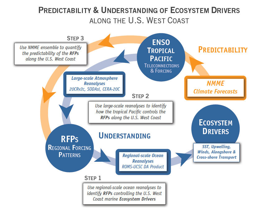
The joint US CLIVAR/OCB/NOAA/PICES/ICES workshop on Forecasting ENSO impacts on marine ecosystems of the US West Coast (Di Lorenzo et al. 2017) held in La Jolla, California, in August 2016 outlined a three-step strategy to better understand and quantify the ENSO-related predictability of marine ecosystem drivers along the US West Coast (Figure 1). The first step is to use a high-resolution ocean reanalysis to determine the association between local ecosystem drivers and regional forcing patterns (RFPs). The identification of ecosystem drivers will depend on the ecosystem indicators or target species selected for prediction (Ohman et al., this issue). The second step is to objectively identify the tropical sea surface temperature (SST) patterns that optimally force the RFPs along the US West Coast region using available long-term large-scale reanalysis products. While the goal of the first two steps is to understand the dynamical basis for predictability (Figure 1, blue path), the final third step (Figure 1, orange path) aims at quantifying the predictability of the RFPs and estimating their prediction skill at seasonal timescales. This third step can be implemented using the output of multi-model ensemble forecasts such as the North America Multi-Model Ensemble (NMME) or by building efficient statistical prediction models such as Linear Inverse Models (LIMs; Newman et al. 2003).

Figure 1. Framework for understanding and predicting ENSO impacts on ecosystem drivers. Blue path shows the steps that will lead to Understanding of the ecosystem drivers and their dependence on tropical Pacific anomalies. Orange path shows the steps that will lead to quantifying the Predictability of marine ecosystem drivers along the US West Coast that are predictable from large-scale tropical teleconnection dynamics.
Important to the concept of ENSO predictability is the realization that the expressions of ENSO are very diverse and cannot be identified with a few indices (Capotondi et al. 2015; Capotondi et al., this issue). In fact, different expressions of sea surface temperature anomalies (SSTa) in the tropics give rise to oceanic and atmospheric teleconnections that generate different coastal impacts in the northeast Pacific. For this reason, we will refer to ENSO as the collection of tropical Pacific SSTa that lead to deterministic and predictable responses in the regional ocean and atmosphere along the US West Coast.
In the sections below, we articulate in more detail the elements of the framework for quantifying the predictability of ENSO-related impacts on coastal ecosystems along the US West Coast (Figure 1). Our focus will be on the California Current System (CCS), reflecting the regional expertise of the workshop participants. Specifically, we discuss (1) the ecosystem drivers and what is identified as such; (2) RFP definitions; and (3) the teleconnections from the tropical Pacific and their predictability.
Ecosystem drivers in the California Current System
The impacts of oceanic processes on the CCS marine ecosystem have been investigated since the 1950s when the long-term California Cooperative Oceanic Fisheries Investigations (CalCOFI) began routine seasonal sampling of coastal ocean waters. The CalCOFI program continues today and has been augmented with several other sampling programs (e.g., the coastal ocean observing network), leading to an unprecedented understanding of how climate and physical ocean processes, such as upwelling, drive ecosystem variability and change (e.g., see more recent reviews from King et al.2011; Ohman et al. 2013; Di Lorenzo et al. 2013).
The dominant physical oceanographic drivers of ecosystem variability occur on seasonal, interannual, and decadal timescales and are associated with changes in (1) SST; (2) upwelling velocity; (3) alongshore transport; (4) cross-shore transport; and (5) thermocline/nutricline depth (see Ohman et al., this issue). This set of ecosystem drivers emerged from discussions among experts at the workshop. Ecosystem responses to these drivers include multiple trophic levels, including phytoplankton, zooplankton, small pelagic fish, and top predators, and several examples have been identified for the CCS (see summary table in Ohman et al., this issue).
While much research has focused on diagnosing the mechanisms by which these physical drivers impact marine ecosystems, less is known about the dynamics controlling the predictability of these drivers. As highlighted in Ohman et al. (this issue), most of the regional oceanographic drivers (e.g., changes in local SST, upwelling, transport, thermocline depth) are connected to changes in large-scale forcings (e.g., winds, surface heat fluxes, large-scale SST and sea surface height patterns, freshwater fluxes, and remotely forced coastally trapped waves entering the CCS from the south). In fact, several studies have documented how large-scale changes in wind patterns associated with the Aleutian Low and the North Pacific Oscillation drive oceanic modes of variability such as the Pacific Decadal Oscillation and the North Pacific Gyre Oscillation (Mantua et al. 1997; Di Lorenzo et al. 2008; Chhak et al. 2009; Ohman et al., this issue; Jacox et al., this issue; Anderson et al., this issue; Capotondi et al., this issue) that influence the CCS. However, these large-scale modes only explain a fraction of the ecosystem’s atmospheric forcing functions at the regional-scale. Thus, it is important to identify other key forcings to gain a more complete mechanistic understanding of CCS ecosystem drivers (e.g., Jacox et al. 2014; 2015).
Atmospheric and oceanic regional forcing patterns
The dominant large-scale quantities that control the CCS ecosystem drivers are winds, heat fluxes, and remotely forced coastally trapped waves (Hickey 1979). Regional expressions or patterns of these large-scale forcings have been linked to changes in local stratification and thermocline depth (Veneziani et al. 2009a; 2009b; Combes et al. 2013), cross-shore transport associated with mesoscale eddies (Kurian et al. 2011; Todd et al. 2012; Song et al. 2012; Davis and Di Lorenzo 2015b), and along-shore transport (Davis and Di Lorenzo 2015a; Bograd et al. 2015). For this reason, we define the regional expressions of the atmospheric and remote wave forcing that are optimal in driving SST, ocean transport, upwelling, and thermocline depth as the RFPs. To clarify this concept, consider the estimation of coastal upwelling velocities. While a change in the position and strength in the Aleutian Low has been related to coastal upwelling in the northern CCS, a more targeted measure of the actual upwelling vertical velocity and nutrient fluxes that are relevant to primary productivity can only be quantified by taking into account a combination of oceanic processes that depend on multiple RFPs such as thermocline depth (e.g., remote waves), thermal stratification (e.g., heat fluxes), mesoscale eddies, and upwelling velocities (e.g., local patterns of wind stress curl and alongshore winds; see Gruber et al 2011; Jacox et al. 2015; Renault et al. 2016). In other words, if we consider the vertical coastal upwelling velocity (w) along the northern CCS, a more adequate physical description and quantification would be given from a linear combination of the different regional forcing functions w = Σn ∝n * RFPn rather than w = ∝*Aleutian Low.
The largest interannual variability in the Pacific that impacts the RFPs is ENSO, which also constitutes the largest source of seasonal (3-6 months) predictability. During El Niño and La Niña, atmospheric and oceanic teleconnections from the tropics modify large-scale and local surface wind patterns and ocean currents of the CCS and force coastally trapped waves.
ENSO teleconnections and potential seasonal predictability of the regional forcing patterns
While ENSO exerts important controls on the RFPs in the CCS, it has become evident that ENSO expressions in the tropics vary significantly from event to event, leading to different responses in the CCS (Capotondi et al., this issue). Also, as previously pointed out, the CCS is not only sensitive to strong ENSO events but more generally responds to a wide range of tropical SSTa variability that is driven by ENSO-type dynamics in the tropical and sub-tropical Pacific. For this reason, we define an “ENSO teleconnection” as any RFP response that is linked to ENSO-type variability in the tropics.
ENSO can influence the upwelling and circulation in the CCS region through both oceanic and atmospheric pathways. It is well known that equatorial Kelvin waves, an integral part of ENSO dynamics, propagate eastward along the Equator and continue both northward (and southward) along the coasts of the Americas as coastally trapped Kelvin waves after reaching the eastern ocean boundary. El Niño events are associated with downwelling Kelvin waves, leading to a deepening of the thermocline, while La Niña events produce a shoaling of the thermocline in the CCS (Simpson 1984; Lynn and Bograd 2002; Huyer et al. 2002; Bograd et al. 2009; Hermann et al. 2009; Miller et al. 2015). The offshore scale of coastal Kelvin waves decreases with latitude, and the waves decay while propagating northward along the coast due to dissipation and radiation of westward propagating Rossby waves. In addition, topography and bathymetry can modify the nature of the waves and perhaps partially impede their propagation at some location. Thus, the efficiency of coastal waves of equatorial origin in modifying the stratification in the CCS is still a matter of debate. To complicate matters, regional wind variability south of the CCS also excites coastally trapped waves, which supplement the tropical source.
In the tropics, SST anomalies associated with ENSO change tropical convection and excite mid-troposphere stationary atmospheric Rossby waves that propagate signals to the extratropics, the so-called atmospheric ENSO teleconnections (Capotondi et al., this issue). Through these atmospheric waves, warm ENSO events favor a deepening and southward shift of the Aleutian Low pressure system that is dominant during winter, as well as changes in the North Pacific Subtropical High that is dominant during spring and summer, resulting in a weakening of the alongshore winds, reduced upwelling, and warmer surface water. These changes are similar to those induced by coastal Kelvin waves of equatorial origin, making it very difficult to distinguish the relative importance of the oceanic and atmospheric pathways in the CCS. In addition, due to internal atmospheric noise, the details of the ENSO teleconnections can vary significantly from event to event and result in important differences along the California Coast (Figure 2).
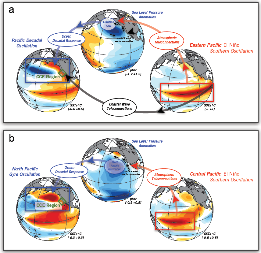
Figure 2. Schematic of ENSO teleconnection associated with different flavors of tropical SSTa. (a) Atmospheric teleconnections of the canonical eastern Pacific El Niño tend to impact the winter expression of the Aleutian Low, which in turn drives an oceanic SSTa anomaly that projects onto the pattern of the Pacific Decadal Oscillation (PDO). (b) Atmospheric teleconnections of the central Pacific El Niño tend to impact the winter expression of the North Pacific High, which in turn drives an oceanic SSTa anomaly that projects onto the pattern of the North Pacific Gyre Oscillation (NPGO). The ENSO SSTa maps are obtained by regressing indices of central and eastern Pacific ENSO with SSTa. The other maps are obtained by regression of SSTa/SLPa with the PDO (a) and NPGO (b) indices.
El Niño events exhibit a large diversity in amplitude, duration, and spatial pattern (Capotondi et al. 2015). The amplitude and location of the maximum SST anomalies, whether in the eastern (EP) or central (CP) Pacific, can have a large impact on ENSO teleconnections (Ashok et al. 2007; Larkin and Harrison 2005). While “canonical” EP events induce changes in the Aleutian Low (Figure 2b), CP events have been associated with a strengthening of the second mode of North Pacific atmospheric variability, the North Pacific Oscillation (NPO; Figure 2a; Di Lorenzo et al. 2010; Furtado et al. 2012). In addition, it is conceivable that EP events have a larger Kelvin wave signature than CP events, resulting in different oceanic influences in the CCS.
In summary, while the ENSO influence on the CCS physical and biological environments is undeniable, several sources of uncertainty remain about the details of that influence. This uncertainty arises in the physical environment on seasonal timescales from many sources, including the diversity of ENSO events, the intrinsic unpredictable components of the atmosphere, and the intrinsic unpredictable eddy variations in the CCS. We also need to distinguish between physically forced ecosystem response versus intrinsic biological variability, which is potentially nonlinear and likely unpredictable. Skill levels need to be quantified for each step of the prediction process (i.e., ENSO, teleconnections, local oceanic response, local ecosystem response) relative to a baseline—for example the persistence of initial condition, which is also being exploited for skillful predictions of the large marine ecosystem at the seasonal timescale (Tommasi et al., this issue). The target populations should be exploitable species that are of interest to federal and state agencies that regulate certain stocks. Models are currently being developed to use ocean forecasts to advance top predator management (Hazen et al., this issue). The implementation of this framework (Figure 1) for practical uses will require a collaborative effort between physical climate scientists with expertise in predicting and understanding ENSO and biologists who have expertise in understanding ecosystem response to physical climate forcing.
Authors
Emanuele Di Lorenzo (Georgia Institute of Technology)
Arthur J. Miller (Scripps Institution of Oceanography)
References
Ashok, K., S.K. Behera, S.A. Rao, H. Weng, and T. Yamagata, 2007: El Niño Modoki and its possible teleconnections. J. Geophys. Res., 112, doi:10.1029/2006JC003798
Bograd, S. J., M. Pozo Buil, E. Di Lorenzo, C. G. Castro, I. D. Schroeder, R. Goericke, C. R. Anderson, C. Benitez-Nelson, and F. A. Whitney, 2015: Changes in source waters to the Southern California Bight. Deep-Sea Res. Part II-Top. Stud. Oceanogr., 112, 42-52, doi:10.1016/j.dsr2.2014.04.009.
Bograd, S. J., I. Schroeder, N. Sarkar, X. Qiu, W. J. Sydeman, and F. B. Schwing, 2009: Phenology of coastal upwelling in the California Current. Geophy. Res. Lett., 36, doi: 10.1029/2008GL035933.
Cai, W. J., and Coauthors, 2015: ENSO and greenhouse warming. Nature Climate Change, 5, 849-859, doi:10.1038/nclimate2743.
Capotondi, A., and Coauthors, 2015: Understanding ENSO Diversity. Bull. Amer. Meteor. Soc., 96, 921-938, doi:10.1175/BAMS-D-13-00117.1.
Chhak, K. C., E. Di Lorenzo, N. Schneider, and P. F. Cummins, 2009: Forcing of low-frequency ocean variability in the northeast Pacific. J. Climate, 22, 1255-1276, doi:10.1175/2008jcli2639.1.
Davis, A., and E. Di Lorenzo, 2015a: Interannual forcing mechanisms of California Current transports I: Meridional Currents. Deep-Sea Res. Part II-Top. Stud. Oceanogr., 112, 18-30, doi:10.1016/j.dsr2.2014.02.005.
Davis, A., and E. Di Lorenzo, 2015b: Interannual forcing mechanisms of California Current transports II: Mesoscale eddies. Deep-Sea Res. Part II-Top. Stud. Oceanogr., 112, 31-41, doi:10.1016/j.dsr2.2014.02.004.
Di Lorenzo, E., and Coauthors, 2017: Forecasting ENSO impacts on marine ecosystems of the US West Coast, Joint US CLIVAR/NOAA/PICES/ICES Report, https://usclivar.org/meetings/2016-enso-ecosystems, forthcoming.
Di Lorenzo, E., and Coauthors, 2008: North Pacific Gyre Oscillation links ocean climate and ecosystem change. Geophys. Res. Lett., 35, doi:10.1029/2007gl032838.
Di Lorenzo, E., and Coauthors, 2013: Synthesis of Pacific Ocean climate and ecosystem dynamics. Oceanogr., 26, 68-81, doi: 10.5670/oceanog.2013.76.
Di Lorenzo, E., K. M. Cobb, J. C. Furtado, N. Schneider, B. T. Anderson, A. Bracco, M. A. Alexander, and D. J. Vimont, 2010: Central Pacific El Nino and decadal climate change in the North Pacific Ocean. Nature Geosci., 3, 762-765, doi:10.1038/ngeo984.
Furtado, J. C., E. Di Lorenzo, B. T. Anderson, and N. Schneider, 2012: Linkages between the North Pacific Oscillation and central tropical Pacific SSTs at low frequencies. Climate Dyn., 39, 2833-2846, doi:10.1007/s00382-011-1245-4.
Gruber, N., Z. Lachkar, H. Frenzel, P. Marchesiello, M. Munnich, J. C. McWilliams, T. Nagai, and G. K. Plattner, 2011: Eddy-induced reduction of biological production in eastern boundary upwelling systems. Nature Geosci., 4, 787-792, doi:10.1038/ngeo1273.
Hermann, A. J., E. N. Curchitser, D. B. Haidvogel, and E. L. Dobbins, 2009: A comparison of remote vs. local influence of El Nino on the coastal circulation of the northeast Pacific. Deep Sea Res. Part II: Top. Stud. Oceanogr., 56, 2427-2443, doi: 10.1016/j.dsr2.2009.02.005.
Hickey, B. M., 1979. The California Current system—hypotheses and facts. Prog. Oceanogr., 8, 191-279, doi: 10.1016/0079-6611(79)90002-8.
Huyer, A., R. L. Smith, and J. Fleischbein, 2002: The coastal ocean off Oregon and northern California during the 1997–8 El Nino. Prog. Oceanogr., 54, 311-341, doi: 10.1016/S0079-6611(02)00056-3.
Jacox, M. G., A. M. Moore, C. A. Edwards, and J. Fiechter, 2014: Spatially resolved upwelling in the California Current System and its connections to climate variability. Geophy. Res. Lett., 41, 3189-3196, doi:10.1002/2014gl059589.
Jacox, M. G., J. Fiechter, A. M. Moore, and C. A. Edwards, 2015: ENSO and the California Current coastal upwelling response. J. Geophy. Res.-Oceans, 120, 1691-1702, doi:10.1002/2014jc010650.
Jacox, M. G., S. J. Bograd, E. L. Hazen, and J. Fiechter, 2015: Sensitivity of the California Current nutrient supply to wind, heat, and remote ocean forcing. Geophys. Res. Lett., 42, 5950-5957, doi:10.1002/2015GL065147.
Jacox, M. G., E. L. Hazen, K. D. Zaba, D. L. Rudnick, C. A. Edwards, A. M. Moore, and S. J. Bograd, 2016: Impacts of the 2015-2016 El Niño on the California Current System: Early assessment and comparison to past events. Geophys. Res. Lett., 43, 7072-7080, doi:10.1002/2016GL069716.
King, J. R., V. N. Agostini, C. J. Harvey, G. A. McFarlane, M. G. G. Foreman, J. E. Overland, E. Di Lorenzo, N. A. Bond, and K. Y. Aydin, 2011: Climate forcing and the California Current ecosystem. Ices J. Mar. Sci., 68, 1199-1216, doi:10.1093/icesjms/fsr009.
Kurian, J., F. Colas, X. Capet, J. C. McWilliams, and D. B. Chelton, 2011: Eddy properties in the California Current System. J. Geophy. Res.-Oceans, 116, doi:10.1029/2010jc006895.
Larkin, N. K. and D. E. Harrison, 2005: On the definition of El Niño and associated seasonal average US weather anomalies. Geophy. Res. Lett. 32, doi: 10.1029/2005GL022738.
Lynn, R. J. and S. J. Bograd, 2002: Dynamic evolution of the 1997–1999 El Niño–La Niña cycle in the southern California Current system. Prog. Oceanogr., 54, 59-75, doi: 10.1016/S0079-6611(02)00043-5.
Mantua, N. J., S. R. Hare, Y. Zhang, J. M. Wallace, and R. C. Francis, 1997: A Pacific interdecadal climate oscillation with impacts on salmon production. Bull. Amer. Meteorol. Soc., 78, 1069-1079, doi:10.1175/1520-0477(1997)078<1069:apicow>2.0.co;2.
Marchesiello, P., J. C. McWilliams, and A. Shchepetkin, 2003: Equilibrium structure and dynamics of the California Current System. J. Phys. Oceanogr., 33, 753-783, doi: 10.1175/1520-0485(2003)33<753:ESADOT>2.0.CO;2.
McCreary, J. P., P. K. Kundu, and S. Y. Chao, 1987: On the dynamics of the California Current System. J. Mar. Res., 45, 1-32, doi: 10.1357/002224087788400945.
Miller, A. J., H. Song, and A. C. Subramanian, 2015: The physical oceanographic environment during the CCE-LTER Years: Changes in climate and concepts. Deep Sea Res. Part II: Top. Stud. Oceanogr., 112, 6-17, doi: 10.1016/j.dsr2.2014.01.003.
Newman, M., and Coauthors, 2016: The Pacific Decadal Oscillation, Revisited. J. Climate, 29, 4399-4427, doi:10.1175/jcli-d-15-0508.1.
Ohman, M. D., K. Barbeau, P. J. S. Franks, R. Goericke, M. R. Landry, and A. J. Miller, 2013: Ecological transitions in a coastal upwelling ecosystem. Oceanogr., 26, 210-219, doi: 10.5670/oceanog.2013.65.
Renault, L., C. Deutsch, J. C. McWilliams, H. Frenzel, J.-H. Liang, and F. Colas, 2016: Partial decoupling of primary productivity from upwelling in the California Current system. Nature Geosci, 9, 505-508, doi:10.1038/ngeo2722.
Simpson, J. J., 1984; El Nino‐induced onshore transport in the California Current during 1982‐1983. Geophy. Res. Lett., 11, 233-236, doi: 10.1029/GL011i003p00233.
Song, H., A. J. Miller, B. D. Cornuelle, and E. Di Lorenzo, 2011: Changes in upwelling and its water sources in the California Current System driven by different wind forcing. Dyn. Atmos. Oceans, 52, 170-191, doi:10.1016/j.dynatmoce.2011.03.001.
Todd, R. E., D. L. Rudnick, M. R. Mazloff, B. D. Cornuelle, and R. E. Davis, 2012: Thermohaline structure in the California Current System: Observations and modeling of spice variance. J. Geophy. Res.-Oceans, 117, doi:10.1029/2011jc007589.
Veneziani, M., C. A. Edwards, J. D. Doyle, and D. Foley, 2009: A central California coastal ocean modeling study: 1. Forward model and the influence of realistic versus climatological forcing. J. Geophy. Res.-Oceans, 114, doi:10.1029/2008jc004774.
Veneziani, M., C. A. Edwards, and A. M. Moore, 2009: A central California coastal ocean modeling study: 2. Adjoint sensitivities to local and remote forcing mechanisms. J. Geophy. Res.-Oceans, 114, doi:10.1029/2008jc004775.

