Ocean Carbon & Biogeochemistry
Studying marine ecosystems and biogeochemical cycles in the face of environmental change
  • Home
  • About OCB
    • About Us
    • Scientific Breadth
      • Biological Pump
      • Changing Marine Ecosystems
      • Changing Ocean Chemistry
      • Estuarine and Coastal Carbon Fluxes
      • Ocean Carbon Uptake and Storage
      • Ocean Observatories
    • Code of Conduct
    • Get Involved
    • Project Office
    • Scientific Steering Committee
    • OCB committees
      • Ocean Time-series
      • US Biogeochemical-Argo
      • Ocean-Atmosphere Interaction
  • Activities
    • Summer Workshop
    • OCB Webinars
    • Guidelines for OCB Workshops & Activities
    • Topical Workshops
      • CMIP6 Models Workshop
      • Coastal BGS Obs with Fisheries
      • C-saw extreme events workshop
      • Expansion of BGC-Argo and Profiling Floats
      • Fish, fisheries and carbon
      • Future BioGeoSCAPES program
      • GO-BCG Scoping Workshop
      • Lateral Carbon Flux in Tidal Wetlands
      • Leaky Deltas Workshop – Spring 2025
      • Marine CDR Workshop
      • Ocean Nucleic Acids ‘Omics
      • Pathways Connecting Climate Changes to the Deep Ocean
    • Small Group Activities
      • Aquatic Continuum OCB-NACP Focus Group
      • Arctic-COLORS Data Synthesis
      • BECS Benthic Ecosystem and Carbon Synthesis WG
      • Carbon Isotopes in the Ocean Workshop
      • CMIP6 WG
      • Filling the gaps air–sea carbon fluxes WG
      • Fish Carbon WG
      • Meta-eukomics WG
      • mCDR
      • Metaproteomic Intercomparison
      • Mixotrophs & Mixotrophy WG
      • N-Fixation WG
      • Ocean Carbonate System Intercomparison Forum
      • Ocean Carbon Uptake WG
      • OOI BGC sensor WG
      • Operational Phytoplankton Observations WG
      • Phytoplankton Taxonomy WG
    • Other Workshops
    • Science Planning
      • Coastal CARbon Synthesis (CCARS)
      • North Atlantic-Arctic
    • Ocean Acidification PI Meetings
    • Training Activities
      • PACE Hackweek 2025
      • PACE Hackweek 2024
      • PACE Training Activity 2022
  • Science Support
    • Data management and archival
    • Early Career
    • Funding Sources
    • Jobs & Postdocs
    • Meeting List
    • OCB Topical Websites
      • Ocean Fertilization
      • Trace gases
      • US IIOE-2
    • Outreach & Education
    • Promoting your science
    • Student Opportunities
    • OCB Activity Proposal Solicitations
      • Guidelines for OCB Workshops & Activities
    • Travel Support
  • Publications
    • OCB Workshop Reports
    • Science Planning and Policy
    • Newsletter Archive
  • Science Highlights
  • News

Archive for Clivar Joint Issue

WBC Series: Observing air-sea interaction in the western boundary currents and their extension regions: Considerations for OceanObs 2019

Posted by mmaheigan 
· Friday, November 10th, 2017 

Dongxiao Zhang1,2, Meghan F. Cronin2, Xiaopei Lin3, Ryuichiro Inoue4, Andrea J. Fassbender5, Stuart P. Bishop6, Adrienne Sutton2

1. University of Washington
2. NOAA Pacific Marine Environmental Laboratory
3. Ocean University of China, China
4. Japan Agency for Marine-Earth Science and Technology, Japan
5. Monterey Bay Aquarium Research Institute
6. North Carolina State University


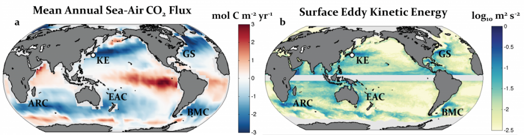
Western boundary currents (WBCs) and their extensions (WBCE) are characterized by intense air-sea heat, momentum, buoyancy, and carbon dioxide (CO2) fluxes (Figure 1a). These large ocean-atmosphere exchanges contribute to the global balance of physical and biogeochemical ocean properties. Excess heat absorbed by the ocean in the tropics is transported poleward, mainly by WBCs (Trenberth and Solomon 1994; Fillenbaum et al. 1997; Zhang et al. 2001; Johns et al. 2011), and then released back to the atmosphere along the WBCs and their extensions in subtropical mid-latitudes at the subtropical and subarctic ocean boundaries (Figure 1a). For this reason, WBC regions are referred to as climatic “hot spots” (Nakamura et al. 2015). Likewise, WBC regions are ocean carbon hot spots, areas of large CO2 uptake that counterbalance the large CO2 outgassing in the tropics (Figure 1b). For OceanObs’09, Cronin et al. (2010) made strong recommendations to include multidisciplinary observations in WBC regional observing systems. The present need for such a system is more urgent than ever. While many open questions remain regarding the role of eddies in ventilation and mode water formation events and their interaction with the biological pump, new technologies are making multidisciplinary observations at these scales more feasible than ever. Use of these new tools during process studies could help to address many of the remaining open questions in WBC regions. OceanObs’19 is two years away, making it timely to review the present observing system for WBC regions and begin strategizing the necessary improvements for the next decade.

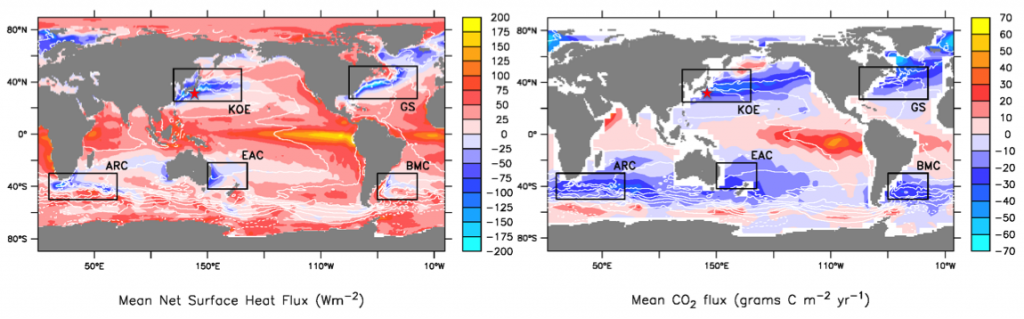
Figure 1. Annual mean air-sea net surface heat flux into the ocean from objectively analyzed flux (OAFlux; Yu and Weller 2007) and sea-to-air surface CO2 flux from Takahashi et al. (2009). White contours are the mean dynamic sea level (Rio and Hernandez 2004); star is the NOAA/PMEL KEO location. The WBC regions in the boxes are the Kuroshio-Oyashio Extension (KOE), Gulf Stream (GS), Brazil and Malvinas Currents (BMC), East Australian Current (EAC), and Agulhas Return Current (ARC). Figure adapted from Cronin et al. (2010).


The following sections briefly describe requirements of the ocean observing system in WBC regions, and how the current or planned observing system is meeting these requirements, such as international partnerships and collaborations. We also briefly discuss some underway process studies and raise some questions that still need to be addressed, by using the Kuroshio Extension observing system as an example that is applicable to other WBC regions. The goal of this article is to motivate discussion for developing future WBC regional observing systems in preparation for OceanObs’19.

Multiscale multidisciplinary air-sea interaction in WBC regions

Following the principles of the Framework for Ocean Observing (Lindstrom et al. 2012), the first step in developing an “observing system that is fit for purpose” is to define the observational requirements of the system, keeping in mind that these can only be fulfilled by an integrated system that spans multiple time and space scales.

A key characteristic of WBC regions is that their intense air-sea fluxes are associated with strong fronts and energized mesoscale and submesoscale eddies. Strong air-sea heat fluxes effectively project the SST front into the atmosphere, potentially affecting storm tracks and mid-latitude weather (Minobe et al. 2008; Small et al. 2008; Kwon et al. 2010). Carbon uptake in the WBCs is largely controlled by physical processes associated with wintertime heat loss that decreases both SST and surface water pCO2 and increases the ocean’s thermodynamic drive to absorb atmospheric CO2. Furthermore, winter heat loss in WBC regions leads to subduction and the formation of mode waters (Qiu et al. 2006; Cronin et al. 2013; Oka et al. 2015) that transport the absorbed CO2 to the ocean interior and act as an important anthropogenic CO2 sink pathway (Sabine et al. 2004). However, the biological pump also plays an important role in determining the magnitude of natural carbon uptake in the transition region between subtropical and subarctic waters (Takahashi et al. 2009; Fassbender et al. 2017; Wakita et al., 2016). Primary production and ecosystem structure and function are strongly regulated by the energetic fronts and (sub)mesoscale eddies associated with WBCs that supply nutrients to the euphotic zone via upwelling (McGillicuddy 2016; Mahadevan 2016; and the references therein) and cross-frontal exchange between high-nutrient, cold subarctic waters and low-nutrient, warm subtropical waters in the upper ocean (Ayers and Lozier 2012; Nagano et al. 2016; Nagai and Clayton 2017). Questions remain about the importance of these biological processes in local anthropogenic carbon uptake relative to other large-scale chemical and physical processes, such as changes in the seawater buffer capacity and mode and intermediate water formation rates. Within the ocean and atmosphere physics communities, it is becoming clear that to properly represent the energy balance of the climate system in a WBC region, it is necessary to resolve the multi-scale ocean and atmosphere interactions, from large-scale to frontal scale to mesoscale, and potentially even submesoscale. As discussed at the recent joint US CLIVAR and Ocean Carbon and Biogeochemistry (OCB) Ocean Carbon Hot Spots workshop, this is less clear for the biogeochemical system. While biological production is clearly sensitive to fronts and eddies – and recent data from the Kuroshio Extension Observatory (KEO) sediment trap show an accumulation peak that can be traced back to a cold-core eddy (M. Honda, pers. comm. 2017) – physical controls of solubility and buffer capacity may be more important for the carbon cycle. Participants of the Ocean Carbon Hot Spots workshop discussed the challenge of quantifying CO2 uptake and understanding air-sea exchange processes in WBC regions in the face of an incomplete observing system and lack of coverage across the fronts and eddies in these systems. Process studies will enable us to examine the complex relationships between air-sea fluxes, eddy activity, mode water formation, physical and biogeochemical properties of mode waters, and primary production. An improved understanding of these physical-chemical-biological interactions can reveal important information about the underlying mechanisms driving low-frequency decadal variations and gyre-scale circulation in WBC regions. These multi-scale, coupled interactions must be considered in the development of a more comprehensive “fit for purpose” WBC regional observing system.

Observing systems of WBC regions

Satellites represent a critical component of all observing systems, delivering global coverage. Because WBC regional fronts are often associated with clouds and rain that can disrupt satellite remote sensing, some remotely sensed fields could have systematic biases in frontal regions. Thus, the WBC regional observing system plan must include efforts to avoid biases and aliasing from improperly resolved fronts and eddies.

Strong currents, winter storms, and warm season typhoons and hurricanes can also make WBC regions challenging for in situ observations. Of all the WBC regions, the Kuroshio Extension currently has the most complete observing system, so we focus on this system as a potential roadmap for other systems.

Kuroshio Extension Observatory: NOAA surface mooring and JAMSTEC sediment trap

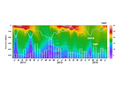
One of the most important observing system components in the Kuroshio Extension is NOAA’s long-term climate reference station, KEO. KEO is strategically located in the Kuroshio Extension recirculation gyre at 32.3°N, 144.5°E (star in Figure 1) on the warm side of the Kuroshio front, an ideal region for monitoring the air-sea interactions that result in mode water formation through winter and spring. Additionally, the site is frequently visited by typhoons during summer and early fall, providing case studies of air-sea interactions between warm water and strong storms. Since 2004, NOAA/PMEL’s Ocean Climate Stations group has maintained a surface mooring at KEO. The NOAA surface mooring measures the meteorological, biogeochemical, and physical ocean variables for estimating air-sea exchanges of heat, moisture, momentum, and carbon dioxide; ocean acidification; and upper ocean variability associated with air-sea interaction. Data are freely available in real time (Figure 2) and are available on GTS (Global Telecommunication System) for improving numerical weather prediction and ocean-atmosphere reanalysis.

Since 2014, Honda et al. (JAMSTEC) have maintained a sediment trap mooring at KEO (Honda pers. comm. 2017). Prior to this, the sediment trap had been deployed at the Japanese S1 mooring, located southeast of KEO at 30°N, 145°E (Honda et al. 2017). The deep sediment trap at 5000 m (800 m above sea floor) positioned next to the KEO surface mooring provides crucial information about the processes affecting nutrient supply that supports ocean productivity and biological carbon export in this subtropical oligotrophic region.

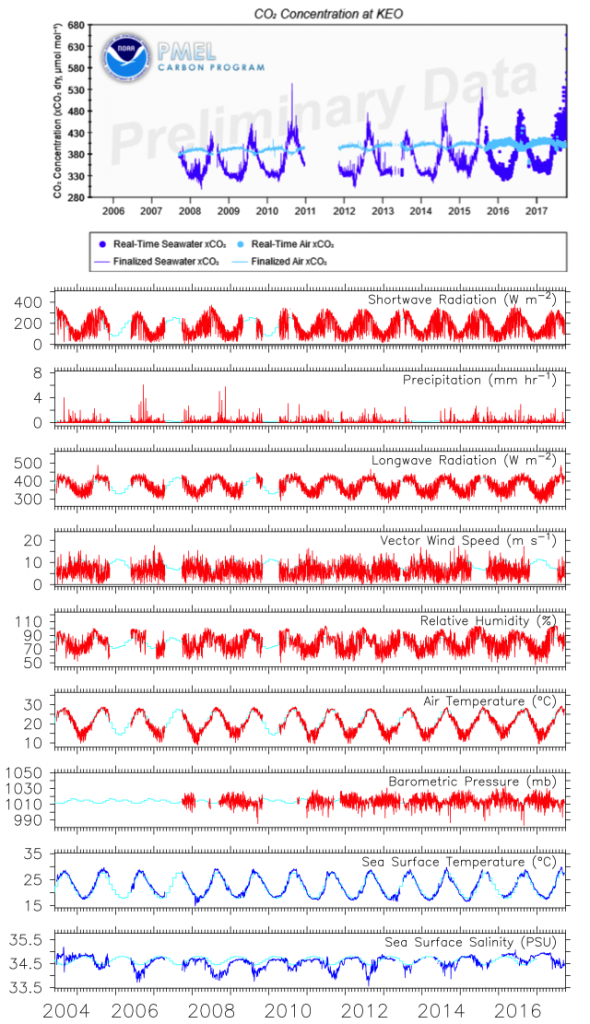
Figure 2. An example of KEO surface observations from real-time data display and delivery web pages.


Japanese-funded process studies JKEO, Hot-Spot, and INBOX

Over the past 13 years, there have been a number of process studies in the Kuroshio Extension region. Most notably, the US-funded Kuroshio Extension System Study (KESS) focused on the dynamics of the mesoscale meanders on the Kuroshio Extension and their interaction with the recirculation gyres north and south of the jet (Jayne et al. 2009; Donohue et al. 2008). This was followed by a study of the effect of the Kuroshio Extension front on the air-sea fluxes and interactions, through deployment of a JAMSTEC-KEO (JKEO) surface mooring north of the Kuroshio Extension front paired with the NOAA KEO mooring south of the front (Konda et al. 2010). Then from 2010 to 2015, the extremely successful Japanese process study, “Multi-Scale Air-Sea Interaction under the East-Asian Monsoon: A ‘Hot Spot’ in the Climate System” (Hot-Spot), led to a large field experiment in the region that included a surface flux mooring K-TRITON buoy deployed closer to the center of the Kuroshio Extension jet, which captured the unusual mesoscale exchanges of water mass properties across the Kuroshio Extension front (Nagano et al. 2016). Another Hot-Spot study with three research vessels, each occupying a half-degree latitude between 35°N-37°N along 143°E and transiting back and forth across the Kuroshio Extension SST front (Kawai et al. 2015), showed unprecedented details of dramatic surface latent and sensible heat flux changes and the response of the deep atmospheric boundary layer across the SST front.

While the Japanese Hot-Spot experiment focused on the physical air-sea interactions, the Japanese Western North Pacific Integrated Physical-Biogeochemical Ocean Observation Experiment (INBOX) (Inoue et al. 2016a) focused on biophysical interactions. In 2011, centered around the S1 mooring in a 150-km box, 18 Argo floats equipped with dissolved oxygen sensors were deployed. In addition, a four-month Seaglider survey was conducted between S1 and KEO in 2014. Results showed a strong association between dissolved oxygen patchiness and mesoscale and submesoscale eddies. With proper coordination through CLIVAR, leveraging international research funding could expand these Japanese-funded experiments.


Chinese KEO buoy

Motivated by recent exciting findings from ultra-high-resolution coupled model simulations showing the importance of latent and sensible heat release from warm ocean eddies in forcing the atmosphere (Ma et al. 2015) and regulating the Kuroshio Extension jet (Ma et al. 2016), the Ocean University of China has successfully deployed an air-sea flux buoy, the Chinese KEO (C-KEO), north of Kuroshio Extension axis at 39ºN, 149.25ºE in October 2017. Similar to KEO, both subsurface and surface measurements at C-KEO will be transmitted and made available to the scientific community in real time when it reaches stable state. In addition, the Ocean University of China has deployed three subsurface moorings (M1: 32.4ºN, 146.2ºE; M2: 39ºN, 150ºE; and M3: 35ºN, 147.6ºE) equipped with ADCP, CTD, a current meter, and McLane Moored Profiler (M1) to monitor the subsurface eddy structure and variability. Over the past three years, they have deployed 19 Argo floats in the Kuroshio Extension region, with a cluster of floats deployed in an anticyclone eddy, providing the detailed eddy contribution to the subduction and mode water formation (Xu et al. 2016). The Qingdao National Laboratory for Marine Science and Technology, as part of its ‘Transparent Ocean’ project, support all of these observing activities.


Challenges and emerging technologies

Characterized by strong winds, high seas, and fast and deep currents, WBC regions are some of the most challenging environments to observe with moored surface buoys. KEO’s long history of success demonstrates that with careful planning, dedication, and international collaborations, sustained moored buoys can be maintained in WBC regions to provide long time series of high-frequency and high-quality simultaneous measurements of subsurface and surface variables. However, due to increased risk of breaking mooring lines in strong, deep jet streams, it is recommended that these long-term reference sites be placed outside of the strongest jet and in the recirculation gyre or northern flank of the jet, like KEO, or the former J-KEO and new C-KEO moorings.

Lagrangian floats have proven to be ideal for studying small-scale fronts and eddies (Shcherbina et al. 2014; Thomas et al. 2017; Inoue et al. 2016b; Xu et al. 2016). Newly available Biogeochemical (BGC)-Argo floats (Johnson and Claustre 2016) may be especially useful for monitoring ocean carbon hot spots to gain a more complete understanding of physical and biogeochemical processes in WBC regions. However, for sustained monitoring and quantifying heat or carbon uptake in eddy-rich WBC regions, a Lagrangian float array would have difficulty to maintain position in strong jets and is susceptible to sampling biases due to the tendency of the floats to be more likely trapped in cyclonic eddies (Rainville et al. 2014; Legg and McWilliams 2002). Controlled surveys by self-propelled autonomous underwater gliders will therefore be necessary to measure moving fronts and eddies and augment moored and Lagrangian components of the observing system.

In situ air-sea flux measurements across fronts and eddies have traditionally required research vessels or voluntary observing ships restricted to limited transit tracks (Fairall et al. 2003; Smith et al. 2016; Palevsky et al. 2016). However, new unmanned surface vehicles (USV) such as Wavegliders (Thompson and Girton 2017) and Saildrones (Meinig et al. 2015; Mordy et al. 2017) are now also being used for air-sea flux measurements of this nature. The Saildrone is especially well suited for collecting observations in the challenging sea conditions of WBC regions. Powered by wind and solar energy with average speed of 3-5 knots (depending on wind, with maximum speed of 7-8 knot), the Saildrone is two times faster than other USVs and has completed a voyage at sea lasting 12 months and covering 16,000 nautical miles. To make the Saildrone capable of observing air-sea exchange processes, NOAA/PMEL, the University of Washington, and Saildrone, Inc. have collaborated to successfully install sensors with equivalent or better quality than those currently used on tropical atmosphere and ocean (TAO) buoys for air-sea flux measurements, as well as a 300 kHz acoustic doppler current profiler (ADCP) for upper ocean current measurements. The standard Saildrone sensor suite also includes: the new PMEL autonomous surface vehicle CO2 system for air-sea CO2 flux measurements; sea surface dissolved oxygen, pH, and chlorophyll sensors; and subsurface backscatter sensing capability from the ADCP, making it a truly interdisciplinary observing platform (Figure 3). Most importantly, Saildrone deployments, measurements, and platform recoveries require no ship time. For example, two Saildrones were recently launched from San Francisco, CA with missions to the eastern tropical Pacific as part of the Tropical Pacific Observing System 2020 project (TPOS2020) and to participate in the field campaign of the NASA Salinity Processes in the Upper Ocean Regional Study (SPURS-2).

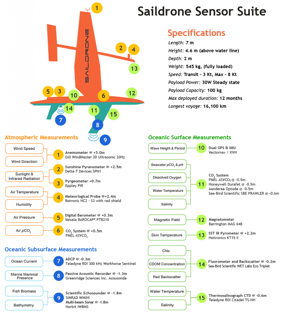
Figure 3. Physical and biogeochemical variables measured by Saildrone.


Conceptual WBC regional observing system for Ocean Obs’19

With uninterrupted satellite measurements of winds, sea surface height, SST, sea surface salinity, precipitation, and ocean color providing a large-scale context of in situ observations, a sustained WBC regional observing system should have the following components to observe multi-scale multidisciplinary processes:

  1. Long-term moored climate reference buoys in the upper ocean equipped with air-sea flux, physical, and biogeochemical sensors and sediment traps, preferably at the opposite flanks of the WBC extension jets
  2. An array of Lagrangian floats, especially BGC-Argo floats, equipped with standard biogeochemical sensors
  3. Underwater gliders for controlled observations of the subsurface ocean and across fronts and eddies
  4. Unmanned surface vehicle sections crossing WBC regional fronts and eddies around and between reference buoys
  5. Underway shipboard measurements including launch of weather balloons when crossing fronts and eddies during float deployments and glider operations


Before such an observing system can be fully developed, process studies are recommended to better understand key physical and biogeochemical processes operating in WBC regions and their associated temporal and spatial scales of variability. Process studies will also inform and optimize the use of newer technologies such as self-navigating platforms together with Lagrangian and Eulerian observations in WBC regions.


Acknowledgements

This is a NOAA PMEL contribution number 4725 and is partially funded by the Joint Institute for the Study of the Atmosphere and Ocean (JISAO) under NOAA Cooperative Agreement and NA15OAR4320063, Contribution No. 2017-0118.


References

Ayers, J. M., and M. S. Lozier, 2012: Unraveling dynamical controls on the North Pacific carbon sink. J. Geophys. Res., 117, doi:10.1029/2011JC007368.

Cronin, M. F., and Coauthors, 2010: Monitoring ocean-atmosphere interactions in western boundary current extensions. In Proceedings of the “OceanObs’09: Sustained Ocean Observations and Information for Society” Conference (Vol. 2), Venice, Italy, 21-25 September 2009, J. Hall, D. E.  Harrison, and D. Stammer, Eds., ESA Publication WPP-306, doi:10.5270/OceanObs09.cwp.20.

Cronin, M. F., N. A. Bond, J. T. Farrar, H. Ichikawa, S. R. Jayne, Y. Kawai, M. Konda, B. Qiu, L. Rainville, and H. Tomita, 2013: Formation and erosion of the seasonal thermocline in the Kuroshio Extension recirculation gyre. Deep-Sea Res. II, 85, 62-74, doi:10.1016/j.dsr2.2012.07.018.

Donohue, K. A., and Coauthors, 2008: Program studies the Kuroshio Extension. Eos, 89, 161-162, doi: 10.1029/2008EO170002.

Fairall, C. W., E. F. Bradley, J. E. Hare, A. A. Grachev and J. B. Edson, 2003: Bulk parameterization of air–sea fluxes: Updates and verification for the COARE algorithm. J. Climate, 16, 571-591, doi: 10.1175/1520-0442(2003)016<0571:BPOASF>2.0.CO;2.

Fassbender, A. J., C. L. Sabine, M. F. Cronin, and A. J. Sutton, 2017: Mixed-layer carbon cycling at the Kuroshio Extension Observatory. Glob. Biogeochem. Cycles, 31, doi:10.1002/2016GB005547.

Fillenbaum, E. R., T. N. Lee, W. E. Johns, and R. Zantopp, 1997: Meridional heat transport variability at 26.5°N in the North Atlantic. J. Phys. Oceanogr., 27, 153–174, doi:10.1175/1520-0485(1997)027<0153:MHTVAN>2.0.CO;2.

Honda, M. C., and Coauthors, 2017a: Comparison of carbon cycle between the western Pacific subarctic and subtropical time-series stations: highlights of the K2S1 project. J. Oceanogr., 73, 647-667, doi:10.1007/s10872-017-0423-3.

Inoue, R., and Coauthors, 2016a: Western North Pacific Integrated Physical-Biogeochemical Ocean Observation Experiment (INBOX): Part 1. Specifications and chronology of the S1-INBOX floats. J. Mar. Res., 74, 43–69, doi:10.1357/002224016819257344.

Inoue, R., V. Faure, and S. Kouketsu, 2016b: Float observations of an anticyclonic eddy off Hokkaido. J. Geophys. Res: Oceans, 121, 6103–6120, doi:10.1002/2016JC011698.

Jayne, S. R., and Coauthors, 2009: The Kuroshio Extension and its recirculation gyres. Deep-Sea Res. I, 56, 2088-2099, doi:10.1016/j.dsr.2009.08.006.

Johns, W. E., and Coauthors, 2011: Continuous, array-based estimates of Atlantic Ocean heat transport at 26.5°N. J. Climate, 24, 2429-2449, doi:10.1175/2010JCLI3997.1.

Johnson, K., and H. Claustre 2016: Bringing biogeochemistry into the Argo age. Eos, 97, doi:10.1029/2016EO062427

Kawai, Y., T. Miyama, S. Iizuka, A. Manda, M. K. Yoshioka, S. Katagiri, Y. Tachibana, and H. Nakamura, 2015: Marine atmospheric boundary layer and low-level cloud responses to the Kuroshio Extension front in the early summer of 2012: three-vessel simultaneous observations and numerical simulations. J. Oceanogr., 71, 511–526, doi:10.1007/s10872-014-0266-0.

Konda, M., H. Ichikawa, H. Tomita, and M. F. Cronin, 2010: Surface heat flux variations across the Kuroshio Extension as observed by surface flux buoys. J. Climate, 23, 5206–5221, doi:10.1175/2010JCLI3391.1.

Kwon, Y.-O., M. A. Alexander, N. A. Bond, C. Frankignoul, H. Nakamura, B. Qiu, L. A. Thompson 2010: Role of the Gulf Stream and Kuroshio–Oyashio Systems in large-scale atmosphere–ocean interaction: A review, J. Climate, 23, 3249-3281, doi: 10.1175/2010JCLI3343.1.

Legg, S., and J. C. McWilliams, 2002: Sampling characteristics from isobaric floats in a convective eddy field. J. Phys. Oceanogr., 32, 527–534, doi:10.1175/1520-0485.

Lindstrom, E. and Coauthors, 2012: A framework for ocean observing. UNESCO, IOC-INF-1284, doi:10.5270/OceanObs09-FOO

Ma, X., P. Chang, R. Saravanan, R. Montuoro, J.-S. Hsieh, D. Wu, X. Lin, L. Wu, and Z. Jing, 2015: Distant influence of Kuroshio Eddies on North Pacific weather patterns? Scient. Rep., 5,  doi:10.1038/srep17785

Ma, X., and Coauthors, 2016: Western boundary currents regulated by interaction between ocean eddies and the atmosphere. Nature, 535, 533–537. doi:10.1038/nature18640

Mahadevan, A. 2016: The impact of submesoscale physics on primary productivity of plankton. Ann. Rev. Mar. Sci., 8, 161-184, doi: 10.1146/annurev-marine-010814-015912.

McGillicuddy, D. J. 2016: Mechanisms of physical-biological-biogeochemical interaction at the oceanic mesoscale. Ann. Rev. Mar. Sci., 8, 125-159, doi: 10.1146/annurev-marine-010814-015606.

Meinig, C., N. Lawrence-Slavas, R. Jenkins, and H.M. Tabisola. 2015: The use of Saildrones to examine spring conditions in the Bering Sea: Vehicle specification and mission performance. OCEANS 2015 – MTS/IEEE Washington. October 19–22, 2015, Washington, DC, 1-6, doi: 10.23919/OCEANS.2015.7404348.

Minobe, S., A. Kuwano-Yoshida, N. Komori, S. P. Xie, and J. R.  Small, 2008: Influence of the Gulf Stream on the troposphere. Nature, 452, 206–209, doi:10.1038/nature06690.

Mordy, C. W., and Coauthors, 2017: Advances in ecosystem research: Saildrone surveys of oceanography, fish, and marine mammals in the Bering Sea. Oceanogr., 30, 113–115, doi: 10.5670/oceanog.2017.230.

Nagai, T., and S. Clayton, 2017: Nutrient interleaving below the mixed layer of the Kuroshio Extension Front. Ocean Dyn., 67, 1027-1046, doi:10.1007/s10236-017-1070-3.

Nagano, A., T. Suga, Y. Kawai, M. Wakita, K. Uehara, and K. Taniguchi, 2016: Ventilation revealed by the observation of dissolved oxygen concentration south of the Kuroshio Extension during 2012–2013. J. Oceanogr., 72, 837–850, doi:10.1007/s10872-016-0386-9.

Nakamura, H., A. Isobe, S. Minobe, H. Mitsudera, M. Nonaka, and T. Suga, 2015: “Hot Spots” in the climate system—new developments in the extratropical ocean–atmosphere interaction research: a short review and an introduction. J. Oceanogr., 71, 463–467, doi:10.1007/s10872-015-0321-5.

Oka, E., B. Qiu, Y. Takatani, K. Enyo, D. Sasano, N. Kosugi, M. Ishii, T. Nakano, and T. Suga, 2015: Decadal variability of subtropical mode water subduction and its impact on biogeochemistry. J. Oceanogr., 71, 389-400, doi: 10.1007/s10872-015-0300-x.

Palevsky, H. I., Quay, P. D., Lockwood, D. E., & Nicholson, D. P. 2016: The annual cycle of gross primary production, net community production, and export efficiency across the North Pacific Ocean. Glob. Biogeochem. Cycles, 30, doi:10.1002/2015GB005318

Qiu, B., P. Hacker, S. Chen, K. A. Donohue, D. R. Watts, H. Mitsudera, N. G. Hogg and S. R. Jayne, 2006: Observations of the subtropical mode water evolution from the Kuroshio Extension System Study. J. Phys. Oceanogr., 36, 457-473, doi:10.1175/JPO2849.1.

Rainville, L., S. R. Jayne, and M. F. Cronin, 2014: Variations of the North Pacific subtropical mode water from direct observations. J. Climate, 27, 2842-2860, doi:10.1175/JCLI-D-13-00227.1.

Rio, M.-H., and F. Hernandez, 2004: A mean dynamic topography computed over the World Ocean from altimetry, in situ measurements, and a geoid model. J. Geophys. Res., 109,  doi:10.1029/2003JC002226.

Sabine, C. L., Feely, R. A., Gruber, N., Key, R. M., Lee, K., Bullister, J. L., Wanninkhof, R., Wong, C., Wallace, D. W. R., Rilbrook, B., Millero, F. J., Peng, T.-H., Kozyr, A., Ono, T., and Rios, A. F., 2004. The oceanic sink for anthropogenic CO2. Science, 305, 367–371, doi:10.1126/science.1097403.

Shcherbina, A. Y., and Coauthors, 2014: The LatMix Summer Campaign: Submesoscale stirring in the upper ocean. Bull. Amer. Meteorol. Soc., 96, 1257–1279, doi:10.1175/BAMS-D-14-00015.1

Small, R. J., S. P. deSzoeke, S. P., Xie, L. O’Neill, H. Seo, Q. Song, Q., P. Cornillon, M. Spall, and S. Minobe, 2008: Air-sea interaction over ocean fronts and eddies. Dyn. Atmos. Oceans, 45, 274–319, doi:10.1016/j.dynatmoce.2008.01.001.

Smith, S. R., N. Lopez, and M. A. Bourassa, 2016: SAMOS air-sea fluxes: 2005–2014. Geosci. Data J., 3, 9-19, doi: 10.1002/gdj3.34.

Takahashi, T., and Coauthors, 2009: Climatological mean and decadal change in surface ocean pCO2, and net sea–air CO2 flux over the global oceans. Deep-Sea Res. Part II: Top. Stud. Oceanogr., 56, 554–577, doi:10.1016/j.dsr2.2008.12.009.

Trenberth, K. E., and A. Solomon 1994: The global heat balance: Heat transports in the atmosphere and ocean, Climate Dyn., 10, 107–134, doi: 10.1007/BF00210625.

Thomas, L. N., J. R. Taylor, E. D’Asaro, C. M. Lee, J. M. Klymak, and A. Shcherbina, 2015: Symmetric instability, inertial oscillations, and turbulence at the Gulf Stream front. J. Phys. Oceanogr., 46, 197–217, doi:10.1175/JPO-D-15-0008.1.

Thomson, J., and J. Girton, 2017: Sustained measurements of Southern Ocean air-sea coupling from a Wave Glider autonomous surface vehicle. Oceanogr., 30, 104–109, doi: 10.5670/oceanog.2017.228.

Wakita, M., and Coauthors, 2016: Biological organic carbon export estimated from the annual carbon budget observed in the surface waters of the western subarctic and subtropical North Pacific Ocean from 2004 to 2013. J. Oceanogr, 72, 1–21. doi:10.1007/s10872-016-0379-8.

Xu, L., P. Li, S.-P. Xie, Q. Liu, Q., C. Liu, and W. Gao, 2016: Observing mesoscale eddy effects on mode-water subduction and transport in the North Pacific. Nature Comm., 7, doi:10.1038/ncomms10505.

Yu, L. and R. A. Weller, 2007: Objectively analyzed air-sea heat fluxes for the global ice-free oceans (1981–2005). Bull. Amer. Meteor. Soc., 88, 527–539, doi: 10.1175/BAMS-88-4-527.

Zhang, D., W. E. Johns, and T. N. Lee 2002: The seasonal cycle of meridional heat transport at 24°N in the North Pacific and in the global ocean. J. Geophys. Res.: Oceans, 107, 1-24, doi:10.1029/2001JC001011


WBC Series: The role of western boundary current regions in the global carbon cycle

Posted by mmaheigan 
· Friday, November 10th, 2017 

Alison R. Gray1, Jaime Palter2

1. University of Washington
2. University of Rhode Island

Estimates of contemporary global air-sea carbon dioxide (CO2) flux (Takahashi et al. 2009; Landschützer et al. 2014) suggest that subtropical western boundary currents (WBCs) and their zonal extensions are key regions of oceanic carbon uptake (Figure 1a). These narrow, intensified currents, which transport water poleward along the western edge of every ocean basin before separating from the continental shelf and turning eastward, are associated with maxima in mean velocity, eddy kinetic energy, air-sea heat flux, and nutrient transport, as well as deep mixed layers on their equatorward flanks. The prominence of these regions in the global air-sea flux of CO2 leads to a basic question: What is the role of the WBCs and their zonal extensions in the global carbon cycle? The answer, which involves the physics and biogeochemistry of the ocean-atmosphere system across a wide range of temporal and spatial scales, reveals the complex nature of these systems and their importance within the climate system, while also highlighting a number of the gaps in our current understanding.

Figure 1: (a) Climatological mean annual sea-air CO2 flux referenced to the year 2000 adapted from Takahashi et al. 2009. Blue (red) areas are ocean sink (source) regions for atmospheric CO2. (b) Surface eddy kinetic energy calculated from the 2011-2013 daily AVISO sea surface height product. The white circle in a and b indicates the location of the Kuroshio Extension Observatory mooring. WBC systems are labeled as follows: Kuroshio Extension (KE), Gulf Stream (GS), Agulhas Return Current (ARC), East Australian Current (EAC), and Brazil-Malvinas Confluence (BMC). Courtesy A. Fassbender and S. Bishop.


Air-sea carbon fluxes are primarily controlled by the difference between the partial pressure of CO2 in the atmosphere, which has been steadily increasing since the 1870s due to the burning of fossil fuels, and the partial pressure of CO2 in seawater (pCO2), which can be influenced by many factors (Sarmiento and Gruber 2006). The contemporary oceanic carbon uptake in the subtropical WBCs and their extensions comes about from both thermally and biologically driven decreases in pCO2. The first of these is tied to the role that WBCs play in the large-scale circulation of the ocean. These currents supply the poleward return flow for the large-scale wind-driven circulation that, through Sverdrup dynamics, generates upper ocean equatorward flow across the vast subtropical gyres (Vallis 2006). As a result, the vigorous (on the order of 1 m s-1) flows in the WBCs rapidly transport warm water from the tropics to mid-latitudes. At mid-latitudes in winter, the atmospheric storm track advects frigid air across the continents and eastward over these warm currents, leading to the largest air-sea heat fluxes in the global ocean. This physical phenomenon has a direct impact on air-sea carbon flux through the solubility effect, whereby ocean cooling reduces pCO2 and thus drives the system towards more uptake by the ocean. The second mechanism for lowering surface ocean pCO2 and producing a flux into the ocean is biological production of organic matter in the euphotic zone, which also occurs at high rates in and around WBCs and their extension regions. This biological productivity is supported by deep convective mixing on the equatorward fringes of the WBCs, which brings nutrients up from the seasonal thermocline, as well as the cross-WBC transport of nutrients. Together these two factors ¾ solubility effects and primary productivity ¾ act to decrease pCO2 in WBCs and their extensions, creating hotspots of ocean carbon uptake.

The impact of air-sea CO2 fluxes on the global climate system hinges on the fate of carbon after it enters the surface ocean, and in this regard, the WBC regions also play a crucial role.  The significant heat loss to the atmosphere and strong winds that combine to create substantial solubility-driven carbon uptake also lead to some of the deepest wintertime mixed layers in the global ocean on the equatorward side of the WBCs. These thick mixed layers are subsequently capped by lighter waters during springtime restratification and then subducted into the ocean interior to form the subtropical mode waters (STMWs) found in each basin. The carbon contained in these mode waters is thus isolated from the atmosphere. How, when, and where STMWs subsequently re-enter the ocean mixed layer governs the influence of WBC carbon uptake on atmospheric carbon concentrations and helps determine the future evolution of the ocean carbon sink (Gruber et al. 2002). Alternatively, carbon taken up in the surface ocean can enter the interior ocean via sinking organic matter that is then remineralized. Depending on the depths to which biological particles sink, this carbon can be trapped below the surface for potentially much longer timescales.

In addition to the role that STMWs play in the transfer of carbon from the surface ocean to the thermocline, the process of mode water formation has several other effects on the oceanic carbon cycle. The deepening of the mixed layer entrains subsurface waters that are higher in dissolved inorganic carbon and nutrients. The resulting increase in mixed layer carbon acts to reduce the pCO2 gradient across the air-sea interface, dampening ocean carbon uptake. The increase in nutrients, however, can also stimulate phytoplankton growth, leading to more biologically driven CO2 uptake. The balance between these processes, which can vary enormously in space and time, will regulate the total carbon uptake and storage in STMWs.  If inorganic carbon and nutrients are entrained into the mixed layer at the same ratio as is removed in sinking organic particles, then primary production will not have a net impact on oceanic CO2 uptake. However, the physical processes that govern both mixed layer dynamics and the upper ocean circulation, as well as the biological processes that determine productivity and export, are frequently decoupled in both space and time. Accordingly, variability in biologically driven carbon uptake can exist on timescales of seasons to decades or longer.

All of the processes described thus far are believed to have been operating since well before anthropogenic perturbations to the atmospheric CO2 concentration. Reconstructions of atmospheric CO2 from ice cores suggest that, averaged over decades, Holocene concentrations were near steady state (Ciais et al. 2013). Therefore, the carbon taken up by the ocean in WBC regions was balanced by outgassing elsewhere, in the climatological mean. The carbon that moves through the climate system through this pre-industrial carbon cycle, referred to as natural carbon, is often conceptually separated from the anthropogenic carbon added to the atmosphere by fossil fuel burning, of which approximately 30% has been absorbed by the ocean (Le Quéré et al. 2016). Modeling and observational studies point to WBCs as being important regions for uptake of anthropogenic carbon, and the STMWs formed on the equatorward flanks of the WBCs account for a significant portion of the anthropogenic carbon storage (Sabine et al. 2004; Iudicone et al., 2016). Climate model-based projections indicate that WBCs and their extensions will continue to be important sinks of carbon as the climate warms (McKinley et al. 2017). However, from observations it is quite difficult to disentangle the natural carbon cycle from the anthropogenic perturbation, and thus natural variability may significantly affect the rates of carbon uptake and storage that we observe.

Together, solubility and biological effects as well as anthropogenic carbon uptake act in concert to create the hotspots of ocean carbon uptake in the WBCs that we observe today. As we become progressively better able to observe and model the climate system, with longer observational records and greater resolution in both space and time, the more variability we find in these highly dynamic regions of the global ocean. WBCs are notable for significant energy at the mesoscale level, i.e., motions at the scales of approximately one month and 100 km at the WBC latitudes, as evidenced by the mean variability in the altimetric sea surface height (Figure 1b). Intense eddying occurs here because WBCs are regions of strong fronts and thus steeply tilted isopycnals. The significant potential energy inherent in this condition leads to the growth of baroclinic instabilities and the substantial mesoscale variability observed in the WBCs.

Mesoscale features can impact the oceanic carbon cycle in a number of different ways. Mesoscale motions strongly affect mixed layer depths, with implications for mode water formation, subduction, and ventilation; the net effect is to increase the stratification of the upper ocean. Many studies have shown that mesoscale eddies, in releasing the potential energy associated with tilted isopycnals, pump heat out of the deep ocean and towards the surface (Gregory 2000; Gnanadesikan et al. 2005; Palter et al. 2014). Given that natural carbon increases with depth in the ocean due to the remineralization of sinking organic matter, this eddy-driven vertical exchange is expected to reduce the strength of the biological pump. On the other hand, anthropogenic carbon concentrations are highest at the ocean’s surface and decrease downward, so that the global-average effect of mesoscale eddies would be expected to decrease the ocean uptake of anthropogenic CO2, relative to an ocean without such eddies.  To infer the current generation of climate models’ ability to represent the net effect of eddies on carbon through common parameterizations, we take cues from an analysis of ocean heat uptake in models of varying resolution (Griffies et al. 2015): Parameterizations were successful in their qualitative representation of the upward transport of heat, albeit at a reduced efficiency relative to the simulations that resolved a rich spectrum of mesoscale eddies. This conclusion suggests that, in the model analyzed, parameterized eddies might underestimate the upward pumping of natural carbon from the ocean interior and overestimate the unbalanced downward transport of anthropogenic carbon by the time-mean circulation.

As a result of the significant horizontal and vertical shear associated with the high levels of mesoscale activity found in the WBCs, these regions are also hotspots of variability at the submesoscales, or motions at scales of approximately 10 km and one day. Such motions, which can be generated through a number of different mechanisms, can be associated with substantial instantaneous vertical velocities and are thought to be critical in the restratification of the mixed layer. Submesoscale motions can lead to strong physical export of particles (Omand et al. 2014), and their effects are only partially parameterized in current generation of climate models.  While a number of ambitious field campaigns have been conducted in recent years in order to better understand these types of motions (e.g., Shcherbina et al. 2015), there are still many open questions regarding the impact of small-scale instabilities on the uptake and storage of carbon through both biophysical coupling and effects on mode water subduction and ventilation.

Diverse physical and biological processes, at a range of temporal and spatial scales, clearly contribute to making the WBCs hotspots of oceanic carbon uptake. While the large-scale mean state of the system is relatively well-understood, a number of challenges remain that currently limit our understanding of the role that WBCs and their extensions play in the global carbon cycle. The spatial and temporal variability in the natural carbon cycle of these systems is not well-characterized, due to the difficulties inherent in both observing and modeling these extremely turbulent regions. Given that the WBC uptake of total carbon (the sum of the natural and anthropogenic components) is determined by the balance of large fluxes both into and out of the ocean, variability in the processes that govern these fluxes can have important effects on the ocean carbon cycle. Although our knowledge of mesoscale and submesoscale physics has increased immensely over the past few decades, how these motions impact biogeochemical cycling at small scales and how these effects feed back on the larger-scale carbon uptake and storage are still open questions. In addition, the Southern Hemisphere WBCs are generally much less studied than their counterparts in the North Atlantic and North Pacific basins, despite the fact that these systems connect to and interact with the Southern Ocean where model estimates indicate approximately 50% of the ocean uptake of anthropogenic carbon has occurred (Frölicher et al. 2015). Indeed, one of the biggest bottlenecks in both quantifying and understanding the role of WBCs in the global carbon cycle remains the chronic scarcity of observations in the Southern Hemisphere.

As we work toward addressing these issues, it remains critically important to develop a mechanistic understanding of the myriad processes that are involved in carbon uptake in the WBCs and their extensions. In this way, we will be able to translate this knowledge into better predictions of future changes in the role of WBCs in the global carbon cycle.


References

Ciais, P., and Coauthors, 2013: Carbon and Other Biogeochemical Cycles. Climate Change 2013: The Physical Science Basis. Contribution of Working Group I to the Fifth Assessment Report of the Intergovernmental Panel on Climate Change, T. F. Stocker, D. Qin, G.-K. Plattner, M. Tignor, S. K. Allen, J. Boschung, A. Nauels, Y. Xia, V. Bex, and P. M. Midgley, Eds., Cambridge University Press, Cambridge, United Kingdom, and New York, USA, doi:10.1017/CBO9781107415324.015.

Frölicher, T. L., J. L. Sarmiento, D. J. Paynter, J. P. Dunne, J. P. Krasting, and M. Winton, 2015: Dominance of the Southern Ocean in anthropogenic carbon and heat uptake in CMIP5 models. J. Climate, 28, 862–886, doi:10.1175/JCLI-D-14-00117.1

Gnanadesikan, A., R. D. Slater, P. S. Swathi, and G. K. Vallis, 2005: The energetics of ocean heat transport, J. Climate, 18, 2604–2616, doi:10.1175/jcli3436.1.

Gregory, J. M., 2000: Vertical heat transports in the ocean and their effect on time-dependent climate change. Climate Dyn., 16, 501-515, doi:10.1007/s003820000059.

Griffies, S. M. and Coauthors, 2015: Impacts on ocean heat from transient mesoscale eddies in a hierarchy of climate models. J. Climate, 28, 952–977, doi:10.1175/JCLI-D-14-00353.1.

Gruber, N., C. D. Keeling, and N. R. Bates, 2002: Interannual variability in the North Atlantic ocean carbon sink. Science, 298, 2374–2378, doi:10.1126/science.1077077.

Iudicone, D., and Coauthors, 2016: The formation of the ocean’s anthropogenic carbon reservoir. Scientific Reports, 6, 35473. http://doi.org/10.1038/srep35473

Landschützer, P., N. Gruber, D. C. E. Bakker, and U. Schuster, 2014: Recent variability of the global ocean carbon sink. Global Biogeochemical Cycles, 28, 927–949. http://doi.org/10.1002/2014GB004853

Le Quéré, C., and Coauthors, 2016: Global Carbon Budget 2016. Earth Syst. Sci. Data., 8, 605-649. DOI:10.5194/essd-8-605-2016.

McKinley, G. A., A. R. Fay, N. S. Lovenduski, and D. J. Pilcher, 2017: Natural variability and anthropogenic trends in the ocean carbon sink. Annu. Rev. Mar. Sci., 9, 125–50. http://doi.org/10.1146/annurev-marine-010816-060529

Omand, M. M., E. A. D’Asaro, C. M. Lee, M. J. Perry, N. Briggs, I. Cetini, and A. Mahadevan, 2015: Eddy-driven subduction exports particulate organic carbon from the spring bloom. Science, 348, 222–225. http://doi.org/10.1126/science.1260062

Palter, J. B., S. M. Griffies, B. L. Samuels, E. D. Galbraith, A. Gnanadesikan, and A. Klocker, 2014: The deep ocean buoyancy budget and its temporal variability. J. Climate, 27, 551–573, doi:10.1175/JCLI-D-13-00016.1.

Sabine, C. L., and Coauthors, 2004: The oceanic sink for anthropogenic CO2. Science, 305, 367–371. http://doi.org/10.1126/science.1097403

Sarmiento, J. L., and N. Gruber, 2006: Ocean Biogeochemical Dynamics. Princeton University Press, New Jersey, USA, ISBN:9781400849079.

Shcherbina, A. Y., and Coauthors, 2015: The LatMix summer campaign: Submesoscale stirring in the upper ocean. Bulletin of the American Meteorological Society, 96, 1257–1279. http://doi.org/10.1175/BAMS-D-14-00015.1

Takahashi, T., and Coauthors, 2009: Climatological mean and decadal change in surface ocean pCO2, and net sea–air CO2 flux over the global oceans. Deep-Sea Res. Part II: Top. Stud. Oceanogr., 56, 554–577, doi:10.1016/j.dsr2.2008.12.009.

Vallis, G. K., 2006: Atmospheric and Oceanic Fluid Dynamics: Fundamentals and Large-Scale Circulation.  Cambridge University Press, Cambridge, UK, ISBN: 9780521849692.

WBC Series: Frontiers in western boundary current research

Posted by mmaheigan 
· Friday, November 10th, 2017 

WBC Series Guest Editors: Andrea J. Fassbender1 and Stuart P. Bishop2

1. Monterey Bay Aquarium Research Institute
2. North Carolina State University

Western boundary current (WBC) regions are often studied for their intensity of air-sea interaction and mesoscale variability, yet research addressing the implications of these characteristics for biogeochemical cycling has lagged behind. WBCs, and their extension jets, display a wide breadth of physical processes that give rise to variability ranging from submesoscale (1-10 km) to basin scale (1000 km). WBC extension jets can act as both barriers and conduits for biological and chemical exchanges between subpolar-subtropical water masses, likely serving an important role in local chemical fluxes and biological community composition. Additionally, WBC regions are known for their formation of subtropical mode waters, carrying their source water biogeochemical signatures into the ocean interior. Interactions between (sub)mesoscale processes, mode water formation, and cross frontal exchanges of chemicals and organisms remain an important and nascent area of research.

In addition to the physical dynamics, many questions remain regarding the role of WBC regions in the global carbon cycle. Recent work suggests that these domains exhibit physically mediated export of biogenic particles and are gateways for anthropogenic carbon injection into the ocean interior. Such recent discovery that WBC processes may be strongly linked to the biological carbon pump and anthropogenic carbon storage speaks to the challenges associated with observing these ocean realms. While much has been learned from pairing satellite remote sensing with in situ physical oceanographic observations, biogeochemical analyses have historically been limited by the lack of necessary observing tools. Thus, there remains a critical knowledge gap on the role of WBCs in the global carbon cycle and other biogeochemical cycles.

With OceanObs’19 approximately two years away, the recent Ocean Carbon Hot Spots workshop assessed community interests and perspectives, revealing that it is an opportune time to make use of novel autonomous observing platforms and biogeochemical sensors to unravel some of the mysteries surrounding the role of WBC extensions in marine biogeochemical cycling. The articles herein present some of the most pressing research questions and observing hurdles related to WBCs from the perspectives of physical, chemical, and biological oceanographers and modelers working in this arena.

Series Articles:

Fine-scale biophysical controls on nutrient supply, phytoplankton community structure, and carbon export in western boundary current regions, S. Clayton, P. Gaube, T. Nagai, M.M. Omand, M. Honda

Decadal variability of the Kuroshio Extension system and its impact on subtropical mode water formation B. Qiu, E. Oka, S.P. Bishop, S. Chen, A.J. Fassbender

Western boundary currents as conduits for the ejection of anthropogenic carbon from the thermocline K.B. Rodgers, P. Zhai, D. Iudicone, O. Aumont, B. Carter, A. J. Fassbender, S. M. Griffies, Y. Plancherel, L. Resplandy, R.D. Slater, K. Toyama

The role of western boundary current regions in the global carbon cycle A.R. Gray, J. Palter

Observing air-sea interaction in the western boundary currents and their extension regions: Considerations for OceanObs 2019 D. Zhang, M.F. Cronin, X. Lin, R. Inoue, A.J. Fassbender, S.P. Bishop, A. Sutton


US CLIVAR Variations Issue PDF (compiled articles)

WBC Series: Western boundary currents as conduits for the ejection of anthropogenic carbon from the thermocline

Posted by mmaheigan 
· Friday, November 10th, 2017 

Keith B. Rodgers1, Ping Zhai1, Daniele Iudicone2, Olivier Aumont3, Brendan Carter4, Andrea J. Fassbender5, Stephen M. Griffies6, Yves Plancherel7, Laure Resplandy8, Richard D. Slater1, Katsuya Toyama9

1. Princeton University
2. Stazione Anton Dohrn, Italy
3. Sorbonne Universités, LOCEAN/IPSL, France
4. University of Washington
5. Monterey Bay Aquarium Research Institute
6. NOAA Geophysical Fluid Dynamics Laboratory
7. University of Oxford, UK
8. Princeton University
9. Japan Meteorological Agency, Japan

A long-standing question regarding the ocean carbon cycle is whether western boundary currents (WBCs) and their extension regions provide an important pathway for anthropogenic carbon (Cant) uptake, thereby contributing to the known importance of these regions in the climate system. Successive versions of the Lamont Doherty Earth Observatory air-sea carbon dioxide (CO2) flux climatologies (Takahashi et al. 2002, 2009) indicate that, at the very least, there is a broad correspondence between the maxima in CO2 fluxes (uptake) and surface heat fluxes (release of heat to the atmosphere over the western subtropical gyres and WBCs). Motivated to understand the mechanistic controls on the ocean carbon cycle in these regions, a number of modeling and observationally based studies have drawn on multiple platforms to constrain fluxes both at the surface and in the interior of this region (Fassbender et al. 2017, and references therein; Nakano et al. 2011).

In particular, Nakano et al. (2015) and Iudicone et al. (2016) have emphasized the value of invoking a density-based framework for understanding the relationship between heat and carbon fluxes in WBCs and their extension regions building on the earlier studies of Iudicone et al. (2008, 2011). Within this framework, WBCs are best understood in the context of the shallow subtropical cell overturning structures (McCreary and Lu 1994; Lu and McCreary 1995) that connect the equatorial upwelling regions with their poleward subtropical water mass formation regions. The role of the subtropical cells in the climate system is to export excess heat absorbed by the coupled system in the equatorial regions to the subtropics, where heat is released along WBCs to the atmosphere. The heat released in WBC regions results in the densification of surface waters and the filling of the subtropical mode water reservoirs. In summary, this overall heat exchange process manifests itself in the ocean as a poleward divergence of warm surface waters in the upper branch of the subtropical cells and a subsurface convergence of cooler thermocline waters. The modeling studies of Nakano et al. (2011, 2015) and Iudicone et al. (2016) argue that the upper branches of the subtropical cells that feed WBCs accumulate Cant over broad scales and that this accumulation is a first-order process in setting the Cant inventory of the subtropical and subpolar mode waters reservoirs. In particular, Nakano et al. (2011) demonstrated that the earlier study of Rodgers et al. (2008), which had argued instead for convection in mode water formation regions to determine Cant uptake, was not supported by the large-scale Lagrangian diagnostics. Although Iudicone et al. (2016) was able to identify an integrated net transfer of Cant to higher density class waters associated with WBCs, given their global focus, they did not consider the specific pathways over which such transfers can occur.

Before proceeding to a mechanistic evaluation of the pathways and mechanisms regulating the transmission of Cant to higher density water masses in WBCs in a global model, it is instructive to first consider a simple budget of Cant over the Southern Hemisphere given by a global ocean carbon cycle model. The model considered is a global non-eddying (nominally 1°) configuration of the Geophysical Fluid Dynamics Laboratory’s (GFDL’s) MOM5-BLING model (Griffies 2012; Galbraith et al. 2011), forced at the surface with CORE-II normal-year forcing (Large and Yeager 2009). The model was spun up for 1000 years, and from 1860-1995 two runs were performed with identical climatological circulation states. For one of the runs, the surface boundary condition for CO2 gas exchange followed observational reconstructions, and for the second run, pre-industrial CO2 was maintained in the atmosphere. Following the definition of Cant of Zhai et al. (2017), who used the same modeling configuration, Cant in the model is the difference between the carbon variables for these two runs. Given our focus on waters for which s0  ≤  27.1, we use potential density for our analysis, following the method presented by Iudicone et al. (2016).


Figure 1. For the Southern Hemisphere, the simulated density-binned inventory of anthropogenic carbon (Cant) in 1995 (solid black), the cumulative air-sea fluxes of Cant over 1861-1995 (dashed black), and the density-binned inventories of Cant from the GLODAPv1 data product of Sabine et al. (2004) (solid blue). For each case, the units are 1015 moles of Cant per Δσ=0.1 kg m-3 density interval.


Figure 1 shows the observationally derived density-binned Cant inventory from the GLODAPv1 product (Sabine et al., 2004) with the density-binned Cant inventories in 1995 and the cumulative air-sea Cant fluxes over 1860-1995 simulated by the model. The cumulative fluxes were density-binned by month and then summed separately for each individual density class over the full period, 1860-1995. The base of the directly ventilated thermocline in the model at 30°S, calculated following the method of Sallée et al. (2013), has been identified to be at s0 = 26.4 in our model configuration. Comparing the density-binned inventories of Cant from GLODAPv1 (Sabine et al. 2004) with the model state in 1995 reveals that the model captures the first-order structure of the total Cant inventories over mode and intermediate waters. This diagnostic view reveals that Cant uptake by gas exchange tends to quantitatively explain storage patterns in waters lighter than the base of the thermocline, as these lighter waters are less likely to be transferred into the interior via subduction. In contrast, in the ocean interior for waters denser than the base of the thermocline, storage tends to exceed uptake (see Iudicone et al. 2016, for a discussion and analytical approximation of these distributions). This is consistent with the idea that WBCs and their extension regions may be serving as “gateways” for the net transfer of Cant from thermocline to sub-thermocline waters.

Figure 2. Maps of fluxes of Cant across the σ0=26.4 horizon for the year 1995, derived using the water mass transformation diagnostics presented in Equations 1 and 2 of Zhai et al. (2017): (a) the buoyancy-driven component, (b) the diffusive transformation term, (c) the contribution from tracer diffusion, and (d) the total diapycnal fluxes. The units are gC m-2 yr-1 and positive values indicate a net transfer from lighter to denser water masses.


In order to identify the specific mechanisms whereby WBCs and their extension regions sustain exchanges between thermocline water masses and subpolar water masses across the base of the thermocline, we consider, for the year 1995, a decomposition into the three dominant drivers in Figure 2. We begin with the contribution from buoyancy exchange with the atmosphere (Figure 2a). The sign convention is such that net buoyancy loss to the atmosphere, resulting in densification of water parcels that contain Cant, results in a positive flux. Thus over the WBCs and their extension regions, the diagnostic reveals a structural and significant annual mean flux of Cant across s0 = 26.4 from subtropical to subpolar water masses (positive), with a smaller flux in the opposing sense from subpolar to subtropical water masses (negative). The diffusive transformation contribution (Figure 2b) reveals a smaller net flux of Cant from subpolar water masses into the thermocline across s0 = 26.4. Thus, this term opposes in its sign the buoyancy-driven component over the WBC and extension regions. A smaller amplitude flux derives from the tracer diffusion contribution (Figure 2c). The total diapycnal flux is shown in Figure 2d, which includes additional terms such as cabbeling – i.e. when two separate water parcels mix to form a third that sinks. Taken together, the results emphasize an interplay of mechanistic drivers over the WBC regions that sustain diapycnal fluxes across the thermocline base and the central importance of heat loss to the atmosphere among the drivers of diapycnal exchanges.

Figure 3. Overturning schematics for the Southern Ocean (three-dimensional domain Y<30°S) for (a) mass fluxes, and (b) for Cant fluxes over the year 1995 in the MOM5-BLING simulation. The coarse graining into thermocline water (TW), subantarctic mode water (SAMW), and Antarctic intermediate water (AAIW) has been accomplished using the algorithmic approach of Sallée et al. (2013). The net freshwater forcing (precipitation minus evaporation, or pme) is shown at the sea surface for the mass fluxes. The mass units are Sverdrups (109 kg s-1) and for Cant are PgC yr-1.


The net cycling of Cant through the ocean’s overturning structures in 1995 can be better appreciated by considering the net transfers between three coarse-grained layers over the Southern Hemisphere:  subtropical thermocline waters (TW) (s0 < 26.4), subantarctic mode water (SAMW), (26.4 < s0 < 27.1), and a deeper layer that will be referred to as Antarctic intermediate water (AAIW) (27.1<s0). Although the deeper layer also aggregates water masses denser than AAIW, our interest is in quantifying fluxes across the SAMW/AAIW interface. For mass (Figure 3a), it can be seen that the principal formation source of SAMW is from AAIW (70%), with only 30% emanating from TW. This stands in stark contrast to the formation sources for Cant in SAMW (Figure 3b), where the TW formation source dominates over the AAIW source within the overturning circulation. In fact, the net of TW-to-SAMW formation sources is of nearly the same amplitude as the net gas exchange uptake of Cant by the SAMW layer over 1995, suggesting highly efficient transfer of Cant to the ocean interior. We wish to emphasize the strong degree of amplification in the TW formation source of Cant relative to mass for SAMW. While the Revelle factor (Revelle and Suess 1957) is expected to contribute to this amplification, a detailed attribution study of the discrepancies between mass and Cant is yet to be realized.

The model results presented here underscore an important role for WBCs and their extension regions in the ejection of Cant from the thermocline into denser waters. Building on the density framework for understanding Cant pathways first developed and presented by Iudicone et al. (2011; 2016), our analyses reveal important net diapycnal transfers of Cant to the ocean interior, consistent with the uptake pathways emphasized in Nakano et al. (2011). Furthermore, these analyses substantiate direct attribution of heat fluxes in WBCs and their extension regions as first-order contributors of Cant storage in sub-thermocline waters associated with the shallow subtropical cell overturning structures.

Ejection of Cant from the thermocline in WBCs and their extension regions has implications for the climate system for two reasons. First, the Revelle factor of low-latitude and thermocline waters is known to be less than that of circumpolar waters (Sabine et al. 2004), meaning that despite higher temperatures, low-latitude waters have an enhanced capacity to absorb Cant from the atmosphere than high-latitude waters. Thus filling a large subpolar reservoir such as SAMW with a subtropical formation source may lead to more efficient storage with respect to a circumpolar formation source. Second, denser subpolar interior water masses are expected to have longer interior renewal or re-emergence timescales for their Cant than subtropical waters (Toyama et al. 2017), and the longer the delay before re-emergence, the weaker the Revelle factor impact will be on regulating future Cant uptake by the ocean. Given the potential significance of the Revelle factor in regulating carbon-climate feedbacks, it will be important to determine whether this entry pathway for Cant might change under future perturbations to the physical state of the ocean.

Viewed in light of the study of Toyama et al. (2017), the net transfer of Cant from thermocline to subpolar water masses across s0=26.4 should be associated with re-emergence of Cant from the thermocline into the ocean’s mixed layer over the Southern Ocean (Toyama et al. 2017). We think it is important to combine the Lagrangian diagnostics for re-emergence applied in that study and the water mass transformation diagnostics applied here within a consistent modeling framework. It is also important to test the sensitivity of the formation sources for the important subtropical and subpolar mode water reservoirs to resolution for eddy-permitting or eddy-resolving model configurations. Of equal importance is the development of new observational constraints on the surface and near-surface formation sources of mode waters, through the development and application of quasi-conservative tracers of water mass transformations. One promising quasi-conservative tracer for this purpose is oceanic radiocarbon, which for the Southern Hemisphere has distinct subtropical and circumpolar surface ocean signatures.


References

Fassbender, A. J., C. L. Sabine, M. F. Cronin, and A. J. Sutton, 2017: Mixed-layer carbon cycling at the Kuroshio Extension Observatory. Global Biogeochem. Cycles, 31, doi:10.1002/2016GB005547.

Galbraith, E. D., and Coauthors, 2011: The impact of climate variability on the distribution of radiocarbon in CM2Mc, a new Earth System Model. J. Climate, 24, 4230-4254, doi:10.1175/2011JCLI3919.1.

Griffies, S. M., 2012: Elements of the Modular Ocean Model (MOM5) (2012 release), GFDL Ocean Group Technical Report No. 7, NOAA/Geophysical Fluid Dynamics Laboratory, 618pp.

Iudicone, D., G. Madec, and T. J. McDougall, 2008: Water-mass transformations in a neutral density framework and the key role of light penetration. J. Phys. Oceanogr., 38, 1357-1376, doi:10.1175/2007JPO3464.1.

Iudicone, D., K. B. Rodgers, I. Stendardo, O. Aumont, G. Madec, L. Bopp, O Mangoni, and M. Ribera d’Alcala, 2011: Water masses as a unifying framework for understanding the Southern Ocean carbon cycle. Biogeosci., 8, 1031-1052,doi:10.5194/bg-8-1031-2011.

Iudicone, D., K. B. Rodgers, Y. Plancherel, O. Aumont, T. Ito, R. M. Key, G. Madec, and M. Ishii, 2016: The formation of the ocean’s anthropogenic carbon reservoir. Sci. Rep., 6, 35473; doi:10.1038/srep35473.

Large, W. G., J. C. McWilliams, and S. C. Doney, 1994: Ocean vertical mixing:  A review and a model with a nonlocal boundary layer parameterization. Rev. Geophys., 32, 363-403, doi:10.1029/94RG01872.

Large, W. G., and S. Yeager, 2009: The global climatology of an interannually varying air-sea flux data set. Climate Dyn.., 33, 341-364, doi:10.1007/s00382-008-0441-3.

Lu, P., and J. P. McCreary, 1995: Influence of the ITCZ on the flow of thermocline water from the subtropical to the equatorial Pacific Ocean. J. Phy. Oceanogr., 25, 3076-3088, doi:10.1175/1520-0485(1995)025<3076:IOTIOT>2.0.CO;2.

McCreary, J. P., and P. Lu, 1994: Interaction between the subtropical and the equatorial ocean circulations: The subtropical cell. J. Phys. Oceanogr., 24, 466-497.

Nakano, H., H. Tsujino, M. Yasuda, T. Hirabara, T. Motoi, M. Ishii, and G. Yamanaka, 2011: Uptake mechanisms of anthropogenic CO2 in the Kuroshio Extension region in an ocean general circulation model. J. Oceanogr., 67, 765-783, doi:10.1007/s10872-011-0075-7.

Nakano, H., M. Ishi, K. B. Rodgers, H. Tsujino, and G. Yamanaka, 2015: Anthropogenic CO2 uptake, transport, storage, and dynamical controls in the ocean imposed by the meridional overturning circulation. Global Biogeochem. Cycles, 29, doi:10.1002/2015GB005128.

Revelle, R., and H. E. Suess, 1957: Carbon dioxide exchange between atmosphere and ocean and the question of an increase of atmospheric CO2 during the past decades. Tellus, 9, 18-27, doi:10.1111j.2153-3490.1957.tb01849.x.

Rodgers, K .B., J. L. Sarmiento, O. Aumont, C. Crevoisier, C. de Boyer Montégut, and N. Metzl, 2008: A wintertime uptake window for anthropogenic CO2 in the North Pacific. Global Biogeochem. Cycles, 22, doi:10.1029/2006GB002920.

Sabine, C., and Coauthors, 2004: The oceanic sink for anthropogenic CO2. Science, 305, 367-371, doi:10.1126/science.1097403.

Sallée, J.-B., E. Schuckburgh, N. Bruneau, A. J. S. Meijers, T. J. Bracegirdle, Z. Wang, and T. Roy, 2013: Assessment of Southern Ocean water mass circulation and characteristics in CMIP5 models:  Historical bias and forcing response. J. Geophys. Res. Oceans, 118, 1830-1844, doi:10.1002/jgrc.20135.

Takahashi, T., S. C. Sutherland, C. Sweeney, A. Poisson, N. Metzl, B. Tilbrook, N. R. Bates, R. Wanninkhof, R. A. Feely, and C. L. Sabine, 2002: Global sea-air CO2 flux based on climatological surface ocean pCO2 and seasonal biological and temperature effects. Deep-Sea Res., Part II, 49, 1601-1622, doi:10.1016/S0967-0645(02)0003-6.

Takahiashi, T., and Coauthors, 2009: Climatological mean and decadal change in surface ocean pCO2 and net sea-air CO2 flux over the global oceans. Deep-Sea Res., Part II, 56, 554-577, doi:10.1016/j.dsr2.2008.12.009.

Toyama, K., K. B. Rodgers, B. Blanke, D. Iudicone, M. Ishii, O. Aumont, and J. L. Sarmiento, 2017: Large re-emergence of anthropogenic carbon into the ocean’s surface mixed layer sustained by the ocean’s overturning circulation. J. Climate, 30, 8615-8631, doi:10.1175/JCLI-D-16-0725.1.

Zhai, P., K. B. Rodgers, S. M. Griffies, R. D. Slater, D. Iudicone, J. L. Sarmiento, and L. Resplandy, 2017: Mechanistic drivers of re-emergence of anthropogenic carbon in the Equatorial Pacific, Geophys. Res. Lett., 44, doi:10.1002/2017GL073758.


WBC Series: Decadal variability of the Kuroshio Extension system and its impact on subtropical mode water formation 

Posted by mmaheigan 
· Friday, November 10th, 2017 

Bo Qiu1, Eitarou Oka2, Stuart P. Bishop3, Shuiming Chen1, Andrea J. Fassbender4

1. University of Hawaii at Manoa
2. The University of Tokyo
3. North Carolina State University
4. Monterey Bay Aquarium Research Institute


After separating from the Japanese coast at 36°N, 141°E, the Kuroshio enters the open basin of the North Pacific, where it is renamed the Kuroshio Extension (KE). Free from the constraint of coastal boundaries, the KE has been observed to be an eastward-flowing inertial jet accompanied by large-amplitude meanders and energetic pinched-off eddies (see Qiu 2002 and Kelly et al. 2010 for comprehensive reviews). Compared to its upstream counterpart south of Japan, the Kuroshio, the KE is accompanied by a stronger southern recirculation gyre that increases the KE’s eastward volume transport to more than twice the maximum Sverdrup transport (~ 60Sv) in the subtropical North Pacific Ocean (Wijffels et al. 1998). This has two important consequences. Dynamically, the increased transport enhances the nonlinearity of the KE jet, rendering the region surrounding the KE jet to have the highest mesoscale activity level in the Pacific basin. Thermodynamically, the enhanced KE jet brings a significant amount of tropical-origin warm water to the mid-latitude ocean to be in direct contact with cold, dry air blowing off the Eurasian continent. This results in significant wintertime heat loss from the ocean to atmosphere surrounding the Kuroshio/KE paths, contributing to the formation of North Pacific subtropical mode water (STMW; see Hanawa and Talley (2001) and Oka and Qiu (2012) for comprehensive reviews).

Figure 1. Yearly paths of the Kuroshio and KE plotted every 14 days using satellite SSH data (updated based on Qiu and Chen 2005). KE was in stable state in 1993–94, 2002–05, and 2010–15, and unstable state in 1995-2001, 2006–09, and 2016, respectively.


Although the ocean is known to be a turbulent medium, variations in both the level of mesoscale eddy activity and the formation rate of STMW in the KE region are by no means random on interannual and longer timescales. One important feature emerging from recent satellite altimeter measurements and eddy-resolving ocean model simulations is that the KE system exhibits clearly defined decadal modulations between a stable and an unstable dynamical state (e.g., Qiu & Chen 2005, 2010; Taguchi et al. 2007; Qiu et al. 2007; Cebollas et al. 2009; Sugimoto and Hanawa 2009; Sasaki et al. 2013; Pierini 2014; Bishop et al. 2015). As shown in Figure 1, the KE paths were relatively stable in 1993–95, 2002–05, and 2010–15. In contrast, spatially convoluted paths prevailed during 1996–2001 and 2006–09. When the KE jet is in a stable dynamical state, satellite altimeter data further reveal that its eastward transport and latitudinal position tend to increase and migrate northward, its southern recirculation gyre tends to strengthen, and the regional eddy kinetic energy level tends to decrease. The reverse is true when the KE jet switches to an unstable dynamical state. In fact, the time-varying dynamical state of the KE system can be well represented by the KE index, defined by the average of the variance-normalized time series of the southern recirculation gyre intensity, the KE jet intensity, its latitudinal position, and the negative of its path length (Qiu et al. 2014). Figure 2a shows the KE index time series in the satellite altimetry period of 1993–present; here, a positive KE index indicates a stable dynamical state and a negative KE index, an unstable dynamical state. From Figure 2a, it is easy to discern the dominance of the decadal oscillations between the two dynamical states of the KE system.

Figure 2. (a) Time series of the KE index from 1993‑present; available at http://www.soest.hawaii.edu/oceanography/bo/KE_index.asc. (b) Year-mean SSH maps when the KE is in stable (2004 and 2011) versus unstable (1997 and 2008) states. (c) SSH anomalies along the zonal band of 32°-34°N from satellite altimetry measurements. (d) Time series of the PDO index from 1989-present; available at http://jisao.washington.edu/pdo/PDO.latest.


Transitions between the KE’s two dynamical states are caused by the basin-scale wind stress curl forcing in the eastern North Pacific related to the Pacific Decadal Oscillation (PDO). Specifically, when the central North Pacific wind stress curl anomalies are positive during the positive PDO phase (see Figure 2d), enhanced Ekman flux divergence generates negative local sea surface height (SSH) anomalies in 170°–150°W along the southern recirculation gyre latitude of 32°–34°N. As these wind-induced negative SSH anomalies propagate westward as baroclinic Rossby waves into the KE region after a delay of 3–4 years (Figure 2c), they weaken the zonal KE jet, leading to an unstable (i.e., negative index) state of the KE system with a reduced recirculation gyre and an active eddy kinetic energy field (Figure 2b). Negative anomalous wind stress curl forcing during the negative PDO phase, on the other hand, generates positive SSH anomalies through the Ekman flux convergence in the eastern North Pacific. After propagating into the KE region in the west, these anomalies stabilize the KE system by increasing the KE transport and by shifting its position northward, leading to a positive index state.

The dynamical state of the KE system exerts a tremendous influence upon the STMW that forms largely along the paths of the Kuroshio/KE jet and inside of its southern recirculation gyre (e.g., Suga et al. 2004; Qiu et al. 2006; Oka 2009). Figure 3a shows the monthly time series of temperature profile, constructed by averaging available Argo and XBT/CTD/XCTD data inside the KE southern recirculation gyre (see Qiu and Chen 2006 for details on the constructing method). The black line in the plot denotes the base of the mixed layer, defined as where the water temperature drops by 0.5°C from the sea surface temperature. Based on the temperature profiles, Figure 3b shows the monthly time series of potential vorticity. STMW in Figure 3b is characterized by water columns with potential vorticity of less than 2.0 x 10⁻¹⁰ m-1s-1 beneath the mixed layer. From Figure 3, it is clear that both the late winter mixed layer depth and the low-potential vorticity STMW layer underwent significant decadal changes over the past 25 years. Specifically, deep mixed layer and pronounced low-potential vorticity STMW were detected in 1993–95, 2001–05, and 2010–15, and these years corresponded roughly to the periods when the KE index was in the positive phase (cf. Figure 2a).


Figure 3. Monthly time series of (a) temperature (°C) and (b) potential vorticity (10-10 m-1 s-1) averaged in the KE’s southern recirculation gyre. The thick black and white lines in (a) and (b) denote the base of the mixed layer, defined as where the temperature drops by 0.5°C from the surface value. Red pluses (at the top of each panel) indicate the individual temperature profiles used in constructing the monthly T(z, t) profiles. The potential vorticity, Q(z,t) = fα∂T(z,t)/∂z, where f is the Coriolis parameter and α the thermal expansion coefficient.


The close connection between the dynamical state of the KE system and the STMW formation has been detected by many recent studies based on different observational data sources and analysis approaches (Qiu and Chen 2006; Sugimoto and Hanawa 2010; Rainville et al. 2014; Bishop and Watts 2014; Oka et al. 2012; 2015; Cerovecki and Giglio 2016). Physically, this connection can be understood as follows. When the KE is in an unstable state (or a negative KE index phase), high-regional eddy variability infuses high-potential vorticity KE and subarctic-gyre water into the southern recirculation gyre, increasing the upper-ocean stratification and hindering the development of deep winter mixed layer and formation of STMW. A stable KE path with suppressed eddy variability (in the positive KE index phase), on the other hand, favors the maintenance of a weak stratification in the recirculation gyre, leading to the formation of a deep winter mixed layer and thick STMW.

Since the STMW is renewed each winter, due to combined net surface heat flux and wind stress forcing that modulate on interannual timescales, a question arising naturally is the timescale on which the dynamical state change of the KE system is able to alter the upper ocean stratification and potential vorticity inside the recirculation gyre. If the influence of the KE dynamical state acts on interannual timescales, one may expect a stronger control on the STMW variability by the wintertime atmospheric condition (e.g., Suga and Hanawa 1995; Davis et al. 2011). Intensive observations from the Kuroshio Extension System Study (KESS) program, spanning the period from April 2004 to July 2006, captured the 2004–05 transition of the KE system from a stable to an unstable state. The combined measurements by profiling Argo floats, moored current meter, current and pressure inverted echo sounder (CPIES), and the Kuroshio Extension Observatory (KEO) surface mooring revealed that the KE dynamical state change was able to change the STMW properties both significantly in amplitude and effectively in time (Qiu et al. 2007; Bishop 2013; Cronin et al. 2013; Bishop and Watts 2014). Relative to 2004, the low-potential vorticity signal in the core of STMW was diminished by one-half in 2005, and this weakening of STMW’s intensity occurred within a period of less than seven months. These significant and rapid responses of STMW to the KE dynamical state change suggests that the variability in STMW formation is more sensitive to the dynamical state of the KE than to interannual variations in overlying atmospheric conditions over the past 25 years.

The decadal variability of STMW in the KE’s southern recirculation gyre is able to affect the water property distributions in the entire western part of the North Pacific subtropical gyre (Oka et al. 2015). Measurements by Argo profiling floats during 2005–14 revealed that the volume and spatial extent of STMW decreased (increased) in 2006–09 (after 2010) during the unstable (stable) KE period in its formation region north of ~28°N, as well as in the southern, downstream regions with a time lag of 1-2 years. Such decadal subduction variability affects not only physical but also biogeochemical structures in the downstream, interior subtropical gyre. Shipboard observations at 25°N and along the 137°E repeat hydrographic section of the Japan Meteorological Agency exhibited that, after 2010, enhanced subduction of STMW consistently increased dissolved oxygen, pH, and aragonite saturation state and decreased potential vorticity, apparent oxygen utilization, nitrate, and dissolved inorganic carbon. Changes in dissolved inorganic carbon, pH, and aragonite saturation state were opposite their long-term trends.

KE State and the Ocean Carbon Cycle

Western boundary current (WBC) regions display the largest magnitude air-to-sea carbon dioxide (CO2) fluxes of anywhere in the global ocean. STMW formation processes are thought to account for a majority of the anthropogenic CO2 sequestration that occurs outside of the polar, deep water formation regions (Sabine et al. 2004; Khatiwala et al. 2009). Once subducted and advected away from the formation region, mode waters often remain out of contact with the atmosphere on timescales of decades to hundreds of years, making them short-term carbon silos relative to the abyssal carbon storage reservoirs. One of the physical impacts on carbon uptake via air-sea CO2 flux is due to the temperature dependence of the solubility of pCO2 in the surface waters. Cooler surface waters during the wintertime months reduce the oceanic pCO2 and subsequently enhance the CO2 flux into the ocean. This carbon uptake corresponds with the timing of peak STMW formation.

As mentioned above, the formation of STMW is modulated by the dynamic states of the KE, with less STMW forming during unstable states and more during stable states. To complicate matters, more enhanced levels of surface chlorophyll (Chla) have also been observed from satellite ocean color during unstable states (Lin et al. 2014), which points to the potential importance of biophysical interactions on carbon uptake. Elevated levels of Chla can further modify the pCO2 of surface waters and enhance carbon export at depth from sinking of particulate organic matter following an individual bloom. Given that submesoscale processes result from deep wintertime mixed layers and from the presence of the larger mesoscale lateral shear and strain fields (McWilliams 2016), it is expected that submesoscale processes are also important in STMW formation during unstable states of the KE. An open question in the research community is to what extent do elevated levels of mesoscale and submesoscale eddy activity modulate STMW formation and carbon uptake during unstable states of the KE? With large variations in STMW formation occurring in concert with decadal variability in the mesoscale eddy field, it is possible that submesoscale processes may impact STMW formation through restratification of the mixed layer within density classes encompassing STMW and timing of the spring bloom. These mesoscale and submesoscale processes may then also impact the uptake of CO2 in the North Pacific on interannual to decadal timescales.


References

Bishop, S. P., 2013: Divergent eddy heat fluxes in the Kuroshio Extension at 143°-149°E. Part II: Spatiotemporal variability. J. Phys. Oceanogr., 43, 2416-2431, doi: 10.1175/JPO-D-13-061.1.

Bishop, S. P., and D. R. Watts, 2014: Rapid eddy-induced modification of subtropical mode water during the Kuroshio Extension System Study. J. Phys. Oceanogr., 44, 1941-1953, doi:10.1175/JPO-D-13-0191.1.

Bishop, S. P., F. O. Bryan, and R. J. Small, 2015: Bjerknes-like compensation in the wintertime north Pacific. J. Phys. Oceanogr., 45, 1339-1355, doi:10.1175/JPO-D-14-0157.1.

Ceballos, L., E. Di Lorenzo, C. D. Hoyos, N. Schneider, and B. Taguchi, 2009: North Pacific Gyre oscillation synchronizes climate variability in the eastern and western boundary current systems. J. Climate, 22, 5163-5174, doi:10.1175/2009JCLI2848.1.

Cerovecki, I., and D. Giglio, 2016: North Pacific subtropical mode water volume decrease in 2006–09 estimated from Argo observations: Influence of surface formation and basin-scale oceanic variability. J. Climate, 29, 2177-2199, doi:10.1175/JCLI-D-15-0179.1.

Cronin, M. F., N. A. Bond, J. T. Farrar, H. Ichikawa, S. R. Jayne, Y. Kawai, M. Konda, B. Qiu, L. Rainville, and H. Tomita, 2013: Formation and erosion of the seasonal thermocline in the Kuroshio Extension Recirculation Gyre. Deep-Sea Res. II, 85, 62-74, doi:10.1016/j.dsr2.2012.07.018.

Davis, X. J., L. M. Rothstein, W. K. Dewar, and D. Menemenlis, 2011: Numerical investigations of seasonal and interannual variability of North Pacific subtropical mode water and its implications for Pacific climate variability. J. Climate, 24, 2648-2665, doi:10.1175/2010JCLI3435.1.

Hanawa, K., and L. D. Talley, 2001: Mode waters. Ocean Circulation and Climate: Observing and Modelling the Global Ocean, G. Siedler, J. Church, and J. Gould, Eds., Academic Press, 373-386.

Khatiwala, S., Primeau, F., and Hall, T., 2009: Reconstruction of the history of anthropogenic CO2 concentrations in the ocean. Nature, 462, 346–349, doi:10.1038/nature08526.

Kelly, K. A., R. J. Small, R. M. Samelson, B. Qiu, T. M. Joyce, Y.-O. Kwon, and M. F. Cronin, 2010: Western boundary currents and frontal air-sea interaction: Gulf Stream and Kuroshio Extension. J. Climate, 23, 5644-5667, doi:10.1175/2010JCLI3346.1.

Lin, P., F. Chai, H. Xue, and P. Xiu, 2014: Modulation of decadal oscillation on surface chlorophyll in the Kuroshio Extension. J. Geophys. Res., 119, 187–199, doi:10.1002/2013JC009359.

McWilliams, J. C., 2016: Submesoscale currents in the ocean. Proc. Roy. Soc. A, 472, doi:10.1098/rspa.2016.0117..

Oka, E., 2009: Seasonal and interannual variation of North Pacific subtropical mode water in 2003–2006. J. Oceanogr., 65, 151-164, doi:10.1007/s10872-009-0015-y.

Oka, E., and B. Qiu, 2012: Progress of North Pacific mode water research in the past decade. J. Oceanogr., 68, 5-20, doi:10.1007/s10872-011-0032-5.

Oka, E., B. Qiu, S. Kouketsu, K. Uehara, and T. Suga, 2012: Decadal seesaw of the central and subtropical mode water formation associated with the Kuroshio Extension variability. J. Oceanogr., 68, 355-360, doi: 10.1007/s10872-015-0300-x.

Oka, E., B. Qiu, Y. Takatani, K. Enyo, D. Sasano, N. Kosugi, M. Ishii, T. Nakano, and T. Suga, 2015: Decadal variability of subtropical mode water subduction and its impact on biogeochemistry. J. Oceanogr., 71, 389-400, doi: 10.1007/s10872-015-0300-x.

Pierini, S., 2014: Kuroshio Extension bimodality and the North Pacific Oscillation: A case of intrinsic variability paced by external forcing. J. Climate, 27, 448-454, doi:10.1175/JCLI-D-13-00306.1.

Qiu, B., 2002: The Kuroshio Extension system: Its large-scale variability and role in the midlatitude ocean-atmosphere interaction. J. Oceanogr., 58, 57-75, doi:10.1023/A:1015824717293.

Qiu, B., and S. Chen, 2005: Variability of the Kuroshio Extension jet, recirculation gyre and mesoscale eddies on decadal timescales. J. Phys. Oceanogr., 35, 2090-2103, doi: 10.1175/JPO2807.1.

Qiu, B., and S. Chen, 2006: Decadal variability in the formation of the North Pacific subtropical mode water: Oceanic versus atmospheric control. J. Phys. Oceanogr., 36, 1365-1380, doi: 10.1175/JPO2918.1.

Qiu, B., and S. Chen, 2010: Eddy-mean flow interaction in the decadally-modulating Kuroshio Extension system. Deep-Sea Res. II, 57, 1098-1110, doi:10.1016/j.dsr2.2008.11.036.

Qiu, B., S. Chen, and P. Hacker, 2007: Effect of mesoscale eddies on subtropical mode water variability from the Kuroshio Extension System Study (KESS). J. Phys. Oceanogr., 37, 982-1000, doi:10.1175/JPO3097.1.

Qiu, B., N. Schneider, and S. Chen, 2007: Coupled decadal variability in the North Pacific: An observationally-constrained idealized model. J. Climate, 20, 3602-3620, doi:10.1175/JCLI4190.1.

Qiu, B., S. Chen, N. Schneider, and B. Taguchi, 2014: A coupled decadal prediction of the dynamic state of the Kuroshio Extension system. J. Climate, 27, 1751-1764, doi:10.1175/JCLI-D-13-00318.1.

Qiu, B., P. Hacker, S. Chen, K. A. Donohue, D. R. Watts, H. Mitsudera, N. G. Hogg and S. R. Jayne, 2006: Observations of the subtropical mode water evolution from the Kuroshio Extension System Study. J. Phys. Oceanogr., 36, 457-473, doi:10.1175/JPO2849.1.

Rainville, L., S. R. Jayne, and M. F. Cronin, 2014: Variations of the North Pacific subtropical mode water from direct observations. J. Climate, 27, 2842-2860, doi:10.1175/JCLI-D-13-00227.1.

Sabine, C. L., Feely, R. A., Gruber, N., Key, R. M., Lee, K., Bullister, J. L., Wanninkhof, R., Wong, C., Wallace, D. W. R., Rilbrook, B., Millero, F. J., Peng, T.-H., Kozyr, A., Ono, T., and Rios, A. F., 2004. The oceanic sink for anthropogenic CO2. Science, 305, 367–371.

Sasaki, Y. N, S. Minobe, and N. Schneider, 2013: Decadal response of the Kuroshio Extension jet to Rossby waves: Observation and thin-jet theory. J. Phys. Oceanogr., 43, 442-456, doi:10.1175/JPO-D-12-096.1.

Suga, T., and K. Hanawa, 1995: Interannual variations of North Pacific subtropical mode water in the 137°E section. J. Phys. Oceanogr., 25, 1012–1017, doi:10.1175/1520-0485(1995)025<1012:IVONPS>2.0.CO;2.

Suga, T., K. Motoki, Y. Aoki, and A. M. MacDonald, 2004: The North Pacific climatology of winter mixed layer and mode waters. J. Phys. Oceanogr., 34, 3–22, doi:10.1175/1520-0485(2004)034<0003:TNPCOW>2.0.CO;2.

Sugimoto, S., and K. Hanawa, 2009: Decadal and interdecadal variations of the Aleutian Low activity and their relation to upper oceanic variations over the North Pacific. J. Meteor. Soc. Japan, 87, 601-614, doi:10.2151/jmsj.87.601.

Sugimoto, S., and K. Hanawa, 2010: Impact of Aleutian Low activity on the STMW formation in the Kuroshio recirculation gyre region. Geophys. Res. Lett., 37, doi:10.1029/ 2009GL041795.

Taguchi, B., S.-P. Xie, N. Schneider, M. Nonaka, H. Sasaki, and Y. Sasai, 2007: Decadal variability of the Kuroshio Extension. Observations and an eddy-resolving model hindcast. J. Climate, 20, 2357-2377, doi:10.1175/JCLI4142.1.

Wijffels, S. E., M. M. Hall, T. Joyce, D. J. Torres, P. Hacker, and E. Firing, 1998: Multiple deep gyres of the western North Pacific: A WOCE section along 149°E. J. Geophys. Res., 103, 12,985-13,009, doi:10.1029/98JC01016.

WBC Series: Fine-scale biophysical controls on nutrient supply, phytoplankton community structure, and carbon export in western boundary current regions

Posted by mmaheigan 
· Friday, November 10th, 2017 

Sophie Clayton1, Peter Gaube1, Takeyoshi Nagai2, Melissa M. Omand3, Makio Honda4

1. University of Washington
2. Tokyo University of Marine Science and Technology, Japan
3. University of Rhode Island
4. Japan Agency for Marine-Earth Science and Technology, Japan

Western boundary current (WBC) regions are largely thought to be hotspots of productivity, biodiversity, and carbon export. The distinct biogeographical characteristics of the biomes bordering WBC fronts change abruptly from stable, subtropical waters to highly seasonal subpolar gyres. The large-scale convergence of these distinct water masses brings different ecosystems into close proximity allowing for cross-frontal exchange. Although the strong horizontal density gradient maintains environmental gradients, instabilities lead to the formation of meanders, filaments, and rings that mediate the exchange of physical, chemical, and ecological properties across the front. WBC systems also act as large-scale conduits, transporting tracers over thousands of kilometers. The combination of these local perturbations and the short advective timescale for water parcels passing through the system is likely the driver of the enhanced local productivity, biodiversity, and carbon export observed in these regions. Our understanding of biophysical interactions in the WBCs, however, is limited by the paucity of in situ observations, which concurrently resolve chemical, biological, and physical properties at fine spatial and temporal scales (1-10 km, days). Here, we review the current state of knowledge of fine-scale biophysical interactions in WBC systems, focusing on their impacts on nutrient supply, phytoplankton community structure, and carbon export. We identify knowledge gaps and discuss how advances in observational platforms, sensors, and models will help to improve our understanding of physical-biological-ecological interactions across scales in WBCs.

Mechanisms of nutrient supply

Nutrient supply to the euphotic zone occurs over a range of scales in WBC systems. The Gulf Stream and the Kuroshio have been shown to act as large-scale subsurface nutrient streams, supporting large lateral transports of nutrients within the upper thermocline (Pelegrí and Csanady 1991; Pelegrí et al. 1996; Guo et al. 2012; Guo et al. 2013). The WBCs are effective in transporting nutrients in part because of their strong volume transports, but also because they support anomalously high subsurface nutrient concentrations compared to adjacent waters along the same isopycnals (Pelegrí and Csanady 1991; Nagai and Clayton 2017; Komatsu and Hiroe pers. comm.). It is likely that the Gulf Stream and Kuroshio nutrient streams originate near the southern boundary of the subtropical gyres (Nagai et al. 2015a). Recent studies have suggested that nutrients in the Gulf Stream originate even farther south in the Southern Ocean (Williams et al. 2006; Sarmiento et al. 2004). These subsurface nutrients can then be supplied to the surface through a range of vertical supply mechanisms, fueling productivity in the WBC regions.

We currently lack a mechanistic understanding of how elevated nutrient levels in these “nutrient streams” are maintained, since mesoscale stirring should act to homogenize them. While it is well understood that the deepening of the mixed layer toward subpolar regions (along nutrient stream pathways) can drive a large-scale induction of nutrients to the surface layer (Williams et al., 2006), the detailed mechanisms driving the vertical supply of these nutrients to the surface layer at synoptic time and space scales remain unclear. Recent studies focusing on the oceanic (sub)mesoscale (spatial scales of 1-100 km) are starting to reveal mechanisms driving intermittent vertical exchange of nutrients and organisms in and out of the euphotic zone.

Recent surveys that resolved micro-scale mixing processes in the Kuroshio Extension and the Gulf Stream have reported elevated turbulence in the thermocline, likely a result of near-inertial internal waves (Nagai et al. 2009, 2012, 2015b; Kaneko et al. 2012, Inoue et al. 2010). In the Tokara Strait, upstream of the Kuroshio Extension, where the geostrophic flow passes shallow topography, pronounced turbulent mixing oriented along coherent banded layers below the thermocline was observed and linked to high-vertical wavenumber near-inertial internal waves (Nagai et al. 2017; Tsutsumi et al. 2017). Within the Kuroshio Extension, measurements made by autonomous microstructure floats have revealed vigorous microscale temperature dissipation within and below the Kuroshio thermocline over at least 300 km following the main stream, which was attributed to active double-diffusive convection (Nagai et al. 2015c). Within the surface mixed layer, recent studies have shown that downfront winds over the Kuroshio Extension generate strong turbulent mixing (D’Asaro et al. 2011; Nagai et al. 2012). The influence of fine-scale vertical mixing on nutrient supply was observed during a high-spatial resolution biogeochemical survey across the Kuroshio Extension front, revealing fine-scale “tongues” of elevated nitrate arranged along isopycnals (Figure 1, Clayton et al. 2014). Subsequent modeling work has shown that these nutrient tongues are ubiquitous features along the southern flank of the Kuroshio Extension front, formed by submesoscale surface mixed layer fronts (Nagai and Clayton 2017).

Microscale turbulence, double-diffusive convection, and submesoscale stirring are all processes associated with meso- and submesoscale fronts. The results from the studies mentioned above support the hypothesis that WBCs are an efficient conduit for transporting nutrients, not only over large scales but also more locally on fine scales, as isopycnal transporters, lateral stirrers, and diapycnal suppliers. It is the sum of these transport processes that ultimately fuels the elevated primary production observed in these regions.

Figure 1. Vertical sections of nitrate (μM) observed across the Kuroshio Extension in October 2009. The panels are organized such that they line up with respect to the density structure of the Kuroshio Extension Front. Cyan contour lines show the mixed layer depth (taken from Nagai and Clayton 2017).

Phytoplankton biomass, community structure, and dynamics

WBCs separate regions with markedly different biogeochemical and ecological characteristics. Subpolar gyres are productive, highly seasonal, tend to support ecosystems with higher phytoplankton biomass, and can be dominated by large phytoplankton and zooplankton taxa. Conversely, subtropical gyres are mostly oligotrophic, support lower photoautotrophic biomass, and are not characterized by a strong seasonal cycle. In turn, these subtropical regions tend to support ecosystems that comprise smaller cells and a tightly coupled microbial loop. As boundaries to these diverse regions, WBCs are the main conduit linking the equatorial and polar oceans and their resident plankton communities. Within the frontal zones, mesoscale dynamics act to stir water masses together and can transport ecosystems across the WBC into regions of markedly different physical and biological characteristics. Furthermore, mesoscale eddies can modulate vertical fluxes via the displacement of ispycnals during eddy intensification or eddy-induced Ekman pumping, or generating submesoscale patches of vertical exchange. At these smaller scales, vigorous vertical circulations ¾ with magnitudes reaching 100 m/day ¾ can fertilize the euphotic zone or transport phytoplankton out of the surface layer.

Numerous studies have hypothesized that the combination of large-scale transport, mesoscale stirring and transport, and submesoscale nutrient input leads to both high biodiversity and high population densities. Using remote sensing data, D’Ovidio et al. (2010) showed that mesoscale stirring in the Brazil-Malvinas Confluence Zone brings together communities from very different source regions, driving locally enhanced biodiversity. In a numerical model, in which physical and biological processes can be explicitly separated and quantified, Clayton et al. (2013) showed that high modeled biodiversity in the WBCs was due to a combination of transport and local nutrient enhancements. And finally, in situ taxonomic surveys crossing the Brazil-Malvinas Confluence (Cermeno et al. 2008) and the Kuroshio Extension (Honjo and Okada 1974; Clayton et al, 2017) showed both enhanced biomass and biodiversity associated with the WBC fronts. Beyond these local enhancements, WBCs might play a larger role in setting regional biogeography. Sugie and Suzuki (2017) found a mixture of temperate and subpolar diatom species in the Kuroshio Extension, suggesting that the boundary current might play a key role in setting downstream diatom diversity.

However tantalizing these results are, they remain relatively inconclusive, in part because of their relatively small temporal and spatial scales. Extending existing approaches for assessing phytoplankton community structure, leveraging emerging ‘omics and continuous sampling techniques, larger regions might be surveyed at high taxonomic and spatial resolution. Combining genomic and transcriptomic observations would provide measures of both organism abundance and activity (Hunt et al. 2013), as well as the potential to better define the relative roles of growth and loss processes. With genetically resolved data and appropriate survey strategies, it will be possible to conclusively determine the presence of these biodiversity hotspots. A better characterization and deeper understanding of these regions will provide insight into the long-term and large-scale biodiversity, stability, and function of the global planktonic ecosystem.

Organic carbon export via physical and biological processes

Export, the removal of fixed carbon from the surface ocean, is driven by gravitational particle sinking, active transport, and (sub)mesoscale processes such as eddy-driven subduction. While evidence suggests that WBCs are likely hot spots of biological (Siegel et al. 2014; Honda et al. 2017a) and physical (Omand et al. 2015) export fluxes out of the euphotic zone, only a small handful of studies have explored this. Recent results from sediment trap studies at the Kuroshio Extension Observatory (KEO) mooring, located just south of the Kuroshio Extension, suggest that there is a link between the passage of mesoscale eddies and carbon export (Honda et al. 2017b). They observed that high export events at 5000 m lagged behind the passage of negative (cyclonic) sea surface height anomalies (SSHA) at the mooring by one to two months (Figure 2). In other regions, underway measurements (Stanley et al. 2010) and optical sensors on autonomous platforms (Briggs et al. 2011; Estapa et al. 2013; Estapa et al. 2015; Bishop et al. 2016) have revealed large episodicity in export proxies over timescales of hours to days and spatial scales of 1-10 km.

Figure 2. Time series of ocean temperature in the upper ~550 m (less than 550 dbar) at station KEO between July 2014 and June 2016. The daily data shown in the figure are available on the KEO database. White contour lines show the temporal variability in the daily satellite-based sea surface height anomaly (SSHA). White open bars show the total mass flux (TMF) observed by the time series sediment trap at 5000 m (based on a figure in Honda et al. 2017b).

Another avenue of carbon export from the surface ocean results from grazing and vertical migration. Vertically migrating zooplankton feed near the surface in the dark and evade predation at depth during the day. Fronts generated by WBCs produce gradients in zooplankton communities, both in terms of grazer biomass and species compositions (e.g., Wiebe and Flierl, 1983), and influence the extent and magnitude of diel vertical migrations. Submesoscale variability in zooplankton abundance can be observed readily in echograms collected by active acoustic sensors, but submesoscale variability in zooplankton community structure and dynamics remains difficult to measure. Thus, the nature of this variability remains largely unknown.

Future research directions

Building a better understanding of how physical and biogeochemical dynamics in WBC regions interact relies on observing these systems at the appropriate scales. This is particularly challenging because of the range of scales at play in these systems and the limitation of existing in situ and remote observing platforms and techniques. As has been outlined above, the ecological and biogeochemical environment of WBCs is the result of long range transport from the flanking subtropical and subpolar gyres, as well as local modification by meso- and submesocale physical dynamics in these frontal systems.

Another challenge in disentangling the relationships between physical and biogeochemical processes in WBCs is the difficulty in measuring rates rather than standing stocks. In such dynamic systems, lags in biological responses mean that the changes in standing stocks may not be collocated with the physical process forcing them. Small-scale lateral stirring spatially and temporally decouples net community production and export while secondary circulations contribute to vertical transport. As much as possible, future process studies should include approaches that can explicitly quantify biological rates and physical transport pathways. New platforms are beginning to fill these observational gaps: BGC-Argo floats, autonomous platforms (e.g., Saildrone), high-frequency underway measurements, and continuous cytometers (including imaging cytometers) are all capable of generating high-spatial resolution datasets of biological and chemical properties over large regions. Gliders and profiling platforms (e.g., WireWalker) are making it possible to measure vertical profiles of biogeochemical properties at high frequency. Operating within a Lagrangian framework, while resolving lateral gradients of physical and biogeochemical tracers with ships or autonomous vehicles, may someday allow us to quantitatively partition the observed small-scale variability in biogeochemical tracers between that attributable to biological or physical processes.


References

Bishop, J. K. B., M. B. Fong, and T. J. Wood, 2016: Robotic observations of high wintertime carbon export in California coastal waters. Biogeosci., 13, 3109-3129, doi:10.5194/bg-13-3109- 2016.

Briggs, N., M. J. Petty, I. Cetinic, I., C. Lee, E. A. Dasaro, A. M. Gray, and E. Rehm, 2011: High-resolution observations of aggregate flux during a subpolar North Atlantic spring bloom. Deep-Sea Res. I, 58, 10311039, doi:10.1016/j.dsr.2011.07.007.

Cermeno, P., S. Dutkiewicz, R. P. Harris, M. Follows, O. Schofield, and P. G. Falkowski, 2008: The role of nutricline depth in regulating the ocean carbon cycle. Proc. Natl. Acad. Sci., 105, 20344-20349. doi:10.1073/pnas.0811302106.

Clayton, S., S. Dutkiewicz, O. Jahn, and M. J. Follows, 2013: Dispersal, eddies, and the diversity of marine phytoplankton. Limn. Ocean. Fluids  Env., 3, 182-197. doi:10.1215/21573689-2373515.

Clayton, S., T. Nagai, and M. J. Follows, 2014: Fine scale phytoplankton community structure across the Kuroshio Front. J. Plankton Res., 36, 1017-1030. doi:10.1093/plankt/fbu020.

Clayton, S., Y.-C. Lin, M. J. Follows, and A. Z. Worden, 2017: Co-existence of distinct Ostreococcus ecotypes at an oceanic front. Limn. Ocean.. 62, 75-88, doi:10.1002/lno.10373.

D’Asaro, E., C. Lee, L. Rainville, L. Harcourt, and L. Thomas, 2011: Enhanced turbulence and energy dissipation at ocean fronts. Science, 332, 318–322, doi: 10.1126/science.1201515.

Estapa, M. L., K. Buesseler, E. Boss, and G. Gerbi, 2013: Autonomous, high-resolution observations of particle flux in the oligotrophic ocean. Biogeosci., 10, 5517-5531, doi: 10.5194/bg-10-5517-2013.

Estapa, M. L., D. A. Siegel, K. O. Buesseler, R. H. R. Stanley, M. W. Lomas, and N. B. Nelson, 2015: Decoupling of net community and export production on submesoscales in the Sargasso Sea. Glob. Biogeochem. Cyc., 29, 12661282, doi:10.1002/2014GB004913.

Guo, X., X.-H. Zhu, Q.-S. Wu, and D. Huang, 2012: The Kuroshio nutrient stream and its temporal variation in the East China Sea. J. Geophys. Res. Oceans, 117, doi:10.1029/2011jc007292.

Guo, X. Y., X. H. Zhu, Y. Long, and D. J. Huang, 2013: Spatial variations in the Kuroshio nutrient transport from the East China Sea to south of Japan. Biogeosci., 10, 6403-6417, doi:10.5194/bg-10-6403-2013.

Honda, M. C., and Coauthors, 2017a: Comparison of carbon cycle between the western Pacific subarctic and subtropical time-series stations: highlights of the K2S1 project. J. Oceanogr., 73, 647-667, doi:10.1007/s10872-017-0423-3.

Honda, M.C., Y. Sasai, E. Siswanto, A. Kuwano-Yoshida, and M. F. Cronin, 2017b: Impact of cyclonic eddies on biogeochemistry in the oligotrophic ocean based on biogeochemical /physical/meteorological time-series at station KEO. Prog. Earth Planet. Sci., submitted.

Honjo, S., and H. Okada, 1974: Community structure of coccolithophores in the photic layer of the mid-Pacific. Micropaleo., 20, 209-230, doi:10.2307/1485061.

Hunt, D. E., Y. Lin, M. J. Church, D. M. Karl, S. G. Tringe, L. K. Izzo, and Z. I. Johnson, 2013: Relationship between abundance and specific activity of bacterioplankton in open ocean surface waters. Appl. Environ. Microbiol., 79, 177-184, doi:10.1128/AEM.02155-12.

Inoue, R., M. C. Gregg, and R. R. Harcourt, 2010: Mixing rates across the Gulf Stream, Part 1: On the formation of Eighteen Degree Water. J. Mar. Res. 68, 643–671.

Kaneko, H., I. Yasuda, K. Komatsu, and S. Itoh, 2012: Observations of the structure of turbulent mixing across the Kuroshio. Geophys. Res. Lett. 39, doi:10.1029/2012GL052419.

Nagai, T., A. Tandon, H. Yamazaki, and M. J. Doubell, 2009: Evidence of enhanced turbulent dissipation in the frontogenetic Kuroshio Front thermocline. Geophys. Res. Lett., 36, doi:10.1029/2009GL038832.

Nagai, T., A. Tandon, H. Yamazaki, M. J. Doubell, and S. Gallager, 2012: Direct observations of microscale turbulence and thermohaline structure in the Kuroshio Front. J. Geophys. Res., 117, doi:10.1029/2011JC007228.

Nagai, T., M. Aiba, and S. Clayton, 2015a: Multiscale route to supply nutrients in the Kuroshio. Kaiyo-to-Seibutsu (In Japanese), 37, 469-477.

Nagai, T., A. Tandon, E. Kunze, and A. Mahadevan, 2015b: Spontaneous generation of near-inertial waves by the Kuroshio Front. J. Phys. Oceanogr., 45, 2381-2406, doi:10.1175/JPO-D-14-0086.1.

Nagai, T., R. Inoue, A. Tandon, and H. Yamazaki, 2015c: Evidence of enhanced double-diffusive convection below the main stream of the Kuroshio Extension.  J. Geophys. Res.,120, 8402-8421, doi: 10.1002/2015JC011288.

Nagai, T., and S. Clayton, 2017: Nutrient interleaving below the mixed layer of the Kuroshio Extension Front. Ocean Dyn., 67, 1027-1046, doi:10.1007/s10236-017-1070-3.

Omand, M. M., M. J. Perry, E. D’Asaro, C. Lee, N. A. Briggs, I. Cetinic, and A. Mahadevan, 2015: Eddy-driven subduction exports particulate organic carbon from the spring bloom. Science, 348, 222–225, doi:10.1126/science.1260062.

d’Ovidio, F., S. De Monte, S. Alvain, Y. Dandonneau, and M. Lévy, 2010: Fluid dynamical niches of phytoplankton types. Proc. Natl. Acad. Sci., 107, 18366-18370. doi:10.1073/pnas.1004620107

Pelegrí, J. L., and G. T. Csanady, 1991: Nutrient transport and mixing in the Gulf Stream. J. Geophys. Res. Oceans, 96, 2577-2583, doi:10.1029/90JC02535.

Pelegrí, J. L., G. T. Csanady, and A. Martins, 1996: The North Atlantic nutrient stream. J. Oceanogr., 52, 275-299, doi: 10.1007/BF02235924.

Sarmiento, J. Á., N. Gruber, M. A. Brzezinski, and J. P. Dunne, 2004: High-latitude controls of thermocline nutrients and low latitude biological productivity. Nature, 427, 56-60, doi:10.1038/nature02127.

Siegel, D. A., K. O. Buesseler, S. C. Doney, S. F. Sailley, M. J. Behrenfeld, and P. W. Boyd, 2014: Global assessment of ocean carbon export by combining satellite observations and food‐web models. Glob. Biogeochem. Cycles, 28, 181-196, doi: 10.1002/2013GB004743.

Stanley, R. H. R., J. B. Kirkpatrick, N. Cassar, B. A. Barnett, and M. L. Bender, 2010: Net community production and gross primary production rates in the western equatorial Pacific: Western equatorial Pacific production. Glob. Biogeochem. Cycles, 24, doi:10.1029/ 2009GB003651.

Sugie, K., and K. Suzuki, 2017: Characterization of the synoptic-scale diversity, biogeography, and size distribution of diatoms in the North Pacific. Limnol. Oceanogr., 62, 884-897, doi:10.1002/lno.10473.

Tsutsumi, E., T. Matsuno, R. C. Lien, H. Nakamura, T. Senjyu, and X. Guo, 2017: Turbulent mixing within the Kuroshio in the Tokara Strait. J. Geophys. Res. Oceans, 122, 7082-7094, doi:10.1002/2017JC013049.

Wiebe, P., and G. Flierl, 1983: Euphausiid invasion/dispersal in Gulf Stream cold-core rings. Mar. Fresh. Res., 34, 625–652, doi: 10.1071/MF9830625.

Williams, R. G., V. Roussenov, and M. J. Follows, 2006: Nutrient streams and their induction into the mixed layer. Glob. Biogeochem. Cycles, 20, doi:10.1029/2005gb002586.


A framework for ENSO predictability of marine ecosystem drivers along the US West Coast

Posted by mmaheigan 
· Thursday, February 16th, 2017 

The US West Coast eastern boundary upwelling system supports one of the most productive marine ecosystems in the world and is a primary source of ecosystem services for the US (e.g., fishing, shipping, and recreation). Long-term historical observations of physical and biological variables in this region have been collected since the 1950s (e.g., the CalCOFI program and now including the coastal ocean observing systems), leading to an excellent foundation for understanding the ecosystem impacts of dominant climate fluctuations such as the El Niño-Southern Oscillation (ENSO). In the northeast Pacific, ENSO impacts a wide range of physical and biotic processes, including temperature, stratification, winds, upwelling, and primary and secondary production. The El Niño phase of ENSO, in particular, can result in extensive geographic habitat range displacements and altered catches of fishes and invertebrates, and impact vertical and lateral export fluxes of carbon and other elements (Jacox et al., this issue; Anderson et al., this issue; Ohman et al., this issue). However, despite empirical observations and increased understanding of the coupling between climate and marine ecosystems along the US West Coast, there has been no systematic attempt to use this knowledge to forecast marine ecosystem responses to individual ENSO events. ENSO forecasting has become routine in the climate community. However, little has been done to forecast the impacts of ENSO on ecosystems and their services. This becomes especially important considering the occurrence of recent strong El Niño events (such as 2015-16) and climate model projections that suggest that ENSO extremes may become more frequent (Cai et al. 2015).

The joint US CLIVAR/OCB/NOAA/PICES/ICES workshop on Forecasting ENSO impacts on marine ecosystems of the US West Coast (Di Lorenzo et al. 2017) held in La Jolla, California, in August 2016 outlined a three-step strategy to better understand and quantify the ENSO-related predictability of marine ecosystem drivers along the US West Coast (Figure 1). The first step is to use a high-resolution ocean reanalysis to determine the association between local ecosystem drivers and regional forcing patterns (RFPs). The identification of ecosystem drivers will depend on the ecosystem indicators or target species selected for prediction (Ohman et al., this issue). The second step is to objectively identify the tropical sea surface temperature (SST) patterns that optimally force the RFPs along the US West Coast region using available long-term large-scale reanalysis products. While the goal of the first two steps is to understand the dynamical basis for predictability (Figure 1, blue path), the final third step (Figure 1, orange path) aims at quantifying the predictability of the RFPs and estimating their prediction skill at seasonal timescales. This third step can be implemented using the output of multi-model ensemble forecasts such as the North America Multi-Model Ensemble (NMME) or by building efficient statistical prediction models such as Linear Inverse Models (LIMs; Newman et al. 2003).

Figure 1. Framework for understanding and predicting ENSO impacts on ecosystem drivers. Blue path shows the steps that will lead to Understanding of the ecosystem drivers and their dependence on tropical Pacific anomalies. Orange path shows the steps that will lead to quantifying the Predictability of marine ecosystem drivers along the US West Coast that are predictable from large-scale tropical teleconnection dynamics.


Important to the concept of ENSO predictability is the realization that the expressions of ENSO are very diverse and cannot be identified with a few indices (Capotondi et al. 2015; Capotondi et al., this issue). In fact, different expressions of sea surface temperature anomalies (SSTa) in the tropics give rise to oceanic and atmospheric teleconnections that generate different coastal impacts in the northeast Pacific. For this reason, we will refer to ENSO as the collection of tropical Pacific SSTa that lead to deterministic and predictable responses in the regional ocean and atmosphere along the US West Coast.

In the sections below, we articulate in more detail the elements of the framework for quantifying the predictability of ENSO-related impacts on coastal ecosystems along the US West Coast (Figure 1). Our focus will be on the California Current System (CCS), reflecting the regional expertise of the workshop participants. Specifically, we discuss (1) the ecosystem drivers and what is identified as such; (2) RFP definitions; and (3) the teleconnections from the tropical Pacific and their predictability.

Ecosystem drivers in the California Current System

The impacts of oceanic processes on the CCS marine ecosystem have been investigated since the 1950s when the long-term California Cooperative Oceanic Fisheries Investigations (CalCOFI) began routine seasonal sampling of coastal ocean waters. The CalCOFI program continues today and has been augmented with several other sampling programs (e.g., the coastal ocean observing network), leading to an unprecedented understanding of how climate and physical ocean processes, such as upwelling, drive ecosystem variability and change (e.g., see more recent reviews from King et al.2011; Ohman et al. 2013; Di Lorenzo et al. 2013).

The dominant physical oceanographic drivers of ecosystem variability occur on seasonal, interannual, and decadal timescales and are associated with changes in (1) SST; (2) upwelling velocity; (3) alongshore transport; (4) cross-shore transport; and (5) thermocline/nutricline depth (see Ohman et al., this issue). This set of ecosystem drivers emerged from discussions among experts at the workshop. Ecosystem responses to these drivers include multiple trophic levels, including phytoplankton, zooplankton, small pelagic fish, and top predators, and several examples have been identified for the CCS (see summary table in Ohman et al., this issue).

While much research has focused on diagnosing the mechanisms by which these physical drivers impact marine ecosystems, less is known about the dynamics controlling the predictability of these drivers. As highlighted in Ohman et al. (this issue), most of the regional oceanographic drivers (e.g., changes in local SST, upwelling, transport, thermocline depth) are connected to changes in large-scale forcings (e.g., winds, surface heat fluxes, large-scale SST and sea surface height patterns, freshwater fluxes, and remotely forced coastally trapped waves entering the CCS from the south). In fact, several studies have documented how large-scale changes in wind patterns associated with the Aleutian Low and the North Pacific Oscillation drive oceanic modes of variability such as the Pacific Decadal Oscillation and the North Pacific Gyre Oscillation (Mantua et al. 1997; Di Lorenzo et al. 2008; Chhak et al. 2009; Ohman et al., this issue; Jacox et al., this issue; Anderson et al., this issue; Capotondi et al., this issue) that influence the CCS. However, these large-scale modes only explain a fraction of the ecosystem’s atmospheric forcing functions at the regional-scale. Thus, it is important to identify other key forcings to gain a more complete mechanistic understanding of CCS ecosystem drivers (e.g., Jacox et al. 2014; 2015).

Atmospheric and oceanic regional forcing patterns

The dominant large-scale quantities that control the CCS ecosystem drivers are winds, heat fluxes, and remotely forced coastally trapped waves (Hickey 1979). Regional expressions or patterns of these large-scale forcings have been linked to changes in local stratification and thermocline depth (Veneziani et al. 2009a; 2009b; Combes et al. 2013), cross-shore transport associated with mesoscale eddies (Kurian et al. 2011; Todd et al. 2012; Song et al. 2012; Davis and Di Lorenzo 2015b), and along-shore transport (Davis and Di Lorenzo 2015a; Bograd et al. 2015). For this reason, we define the regional expressions of the atmospheric and remote wave forcing that are optimal in driving SST, ocean transport, upwelling, and thermocline depth as the RFPs. To clarify this concept, consider the estimation of coastal upwelling velocities. While a change in the position and strength in the Aleutian Low has been related to coastal upwelling in the northern CCS, a more targeted measure of the actual upwelling vertical velocity and nutrient fluxes that are relevant to primary productivity can only be quantified by taking into account a combination of oceanic processes that depend on multiple RFPs such as thermocline depth (e.g., remote waves), thermal stratification (e.g., heat fluxes), mesoscale eddies, and upwelling velocities (e.g., local patterns of wind stress curl and alongshore winds; see Gruber et al 2011; Jacox et al. 2015; Renault et al. 2016). In other words, if we consider the vertical coastal upwelling velocity (w) along the northern CCS, a more adequate physical description and quantification would be given from a linear combination of the different regional forcing functions w = Σn ∝n * RFPn rather than w = ∝*Aleutian Low.

The largest interannual variability in the Pacific that impacts the RFPs is ENSO, which also constitutes the largest source of seasonal (3-6 months) predictability. During El Niño and La Niña, atmospheric and oceanic teleconnections from the tropics modify large-scale and local surface wind patterns and ocean currents of the CCS and force coastally trapped waves.

ENSO teleconnections and potential seasonal predictability of the regional forcing patterns

While ENSO exerts important controls on the RFPs in the CCS, it has become evident that ENSO expressions in the tropics vary significantly from event to event, leading to different responses in the CCS (Capotondi et al., this issue). Also, as previously pointed out, the CCS is not only sensitive to strong ENSO events but more generally responds to a wide range of tropical SSTa variability that is driven by ENSO-type dynamics in the tropical and sub-tropical Pacific. For this reason, we define an “ENSO teleconnection” as any RFP response that is linked to ENSO-type variability in the tropics.

ENSO can influence the upwelling and circulation in the CCS region through both oceanic and atmospheric pathways. It is well known that equatorial Kelvin waves, an integral part of ENSO dynamics, propagate eastward along the Equator and continue both northward (and southward) along the coasts of the Americas as coastally trapped Kelvin waves after reaching the eastern ocean boundary. El Niño events are associated with downwelling Kelvin waves, leading to a deepening of the thermocline, while La Niña events produce a shoaling of the thermocline in the CCS (Simpson 1984; Lynn and Bograd 2002; Huyer et al. 2002; Bograd et al. 2009; Hermann et al. 2009; Miller et al. 2015). The offshore scale of coastal Kelvin waves decreases with latitude, and the waves decay while propagating northward along the coast due to dissipation and radiation of westward propagating Rossby waves. In addition, topography and bathymetry can modify the nature of the waves and perhaps partially impede their propagation at some location. Thus, the efficiency of coastal waves of equatorial origin in modifying the stratification in the CCS is still a matter of debate. To complicate matters, regional wind variability south of the CCS also excites coastally trapped waves, which supplement the tropical source.

In the tropics, SST anomalies associated with ENSO change tropical convection and excite mid-troposphere stationary atmospheric Rossby waves that propagate signals to the extratropics, the so-called atmospheric ENSO teleconnections (Capotondi et al., this issue). Through these atmospheric waves, warm ENSO events favor a deepening and southward shift of the Aleutian Low pressure system that is dominant during winter, as well as changes in the North Pacific Subtropical High that is dominant during spring and summer, resulting in a weakening of the alongshore winds, reduced upwelling, and warmer surface water. These changes are similar to those induced by coastal Kelvin waves of equatorial origin, making it very difficult to distinguish the relative importance of the oceanic and atmospheric pathways in the CCS. In addition, due to internal atmospheric noise, the details of the ENSO teleconnections can vary significantly from event to event and result in important differences along the California Coast (Figure 2).

Figure 2. Schematic of ENSO teleconnection associated with different flavors of tropical SSTa. (a) Atmospheric teleconnections of the canonical eastern Pacific El Niño tend to impact the winter expression of the Aleutian Low, which in turn drives an oceanic SSTa anomaly that projects onto the pattern of the Pacific Decadal Oscillation (PDO). (b) Atmospheric teleconnections of the central Pacific El Niño tend to impact the winter expression of the North Pacific High, which in turn drives an oceanic SSTa anomaly that projects onto the pattern of the North Pacific Gyre Oscillation (NPGO). The ENSO SSTa maps are obtained by regressing indices of central and eastern Pacific ENSO with SSTa. The other maps are obtained by regression of SSTa/SLPa with the PDO (a) and NPGO (b) indices.


El Niño events exhibit a large diversity in amplitude, duration, and spatial pattern (Capotondi et al. 2015). The amplitude and location of the maximum SST anomalies, whether in the eastern (EP) or central (CP) Pacific, can have a large impact on ENSO teleconnections (Ashok et al. 2007; Larkin and Harrison 2005). While “canonical” EP events induce changes in the Aleutian Low (Figure 2b), CP events have been associated with a strengthening of the second mode of North Pacific atmospheric variability, the North Pacific Oscillation (NPO; Figure 2a; Di Lorenzo et al. 2010; Furtado et al. 2012). In addition, it is conceivable that EP events have a larger Kelvin wave signature than CP events, resulting in different oceanic influences in the CCS.

In summary, while the ENSO influence on the CCS physical and biological environments is undeniable, several sources of uncertainty remain about the details of that influence. This uncertainty arises in the physical environment on seasonal timescales from many sources, including the diversity of ENSO events, the intrinsic unpredictable components of the atmosphere, and the intrinsic unpredictable eddy variations in the CCS. We also need to distinguish between physically forced ecosystem response versus intrinsic biological variability, which is potentially nonlinear and likely unpredictable. Skill levels need to be quantified for each step of the prediction process (i.e., ENSO, teleconnections, local oceanic response, local ecosystem response) relative to a baseline—for example the persistence of initial condition, which is also being exploited for skillful predictions of the large marine ecosystem at the seasonal timescale (Tommasi et al., this issue). The target populations should be exploitable species that are of interest to federal and state agencies that regulate certain stocks. Models are currently being developed to use ocean forecasts to advance top predator management (Hazen et al., this issue). The implementation of this framework (Figure 1) for practical uses will require a collaborative effort between physical climate scientists with expertise in predicting and understanding ENSO and biologists who have expertise in understanding ecosystem response to physical climate forcing.

Authors

Emanuele Di Lorenzo (Georgia Institute of Technology)
Arthur J. Miller (Scripps Institution of Oceanography)

References

Ashok, K., S.K. Behera, S.A. Rao, H. Weng, and T. Yamagata, 2007: El Niño Modoki and its possible teleconnections. J. Geophys. Res., 112, doi:10.1029/2006JC003798

Bograd, S. J., M. Pozo Buil, E. Di Lorenzo, C. G. Castro, I. D. Schroeder, R. Goericke, C. R. Anderson, C. Benitez-Nelson, and F. A. Whitney, 2015: Changes in source waters to the Southern California Bight. Deep-Sea Res. Part II-Top. Stud. Oceanogr., 112, 42-52, doi:10.1016/j.dsr2.2014.04.009.

Bograd, S. J., I. Schroeder, N. Sarkar, X. Qiu, W. J. Sydeman, and F. B. Schwing, 2009: Phenology of coastal upwelling in the California Current. Geophy. Res. Lett., 36, doi: 10.1029/2008GL035933.

Cai, W. J., and Coauthors, 2015: ENSO and greenhouse warming. Nature Climate Change, 5, 849-859, doi:10.1038/nclimate2743.

Capotondi, A., and Coauthors, 2015: Understanding ENSO Diversity. Bull. Amer. Meteor. Soc., 96, 921-938, doi:10.1175/BAMS-D-13-00117.1.

Chhak, K. C., E. Di Lorenzo, N. Schneider, and P. F. Cummins, 2009: Forcing of low-frequency ocean variability in the northeast Pacific. J. Climate, 22, 1255-1276, doi:10.1175/2008jcli2639.1.

Davis, A., and E. Di Lorenzo, 2015a: Interannual forcing mechanisms of California Current transports I: Meridional Currents. Deep-Sea Res. Part II-Top. Stud. Oceanogr., 112, 18-30, doi:10.1016/j.dsr2.2014.02.005.

Davis, A., and E. Di Lorenzo, 2015b: Interannual forcing mechanisms of California Current transports II: Mesoscale eddies. Deep-Sea Res. Part II-Top. Stud. Oceanogr., 112,  31-41, doi:10.1016/j.dsr2.2014.02.004.

Di Lorenzo, E., and Coauthors, 2017: Forecasting ENSO impacts on marine ecosystems of the US West Coast, Joint US CLIVAR/NOAA/PICES/ICES Report, https://usclivar.org/meetings/2016-enso-ecosystems, forthcoming.

Di Lorenzo, E., and Coauthors, 2008: North Pacific Gyre Oscillation links ocean climate and ecosystem change. Geophys. Res. Lett., 35, doi:10.1029/2007gl032838.

Di Lorenzo, E., and Coauthors, 2013: Synthesis of Pacific Ocean climate and ecosystem dynamics. Oceanogr., 26, 68-81, doi: 10.5670/oceanog.2013.76.

Di Lorenzo, E., K. M. Cobb, J. C. Furtado, N. Schneider, B. T. Anderson, A. Bracco, M. A. Alexander, and D. J. Vimont, 2010: Central Pacific El Nino and decadal climate change in the North Pacific Ocean. Nature Geosci., 3, 762-765, doi:10.1038/ngeo984.

Furtado, J. C., E. Di Lorenzo, B. T. Anderson, and N. Schneider, 2012: Linkages between the North Pacific Oscillation and central tropical Pacific SSTs at low frequencies. Climate Dyn., 39, 2833-2846, doi:10.1007/s00382-011-1245-4.

Gruber, N., Z. Lachkar, H. Frenzel, P. Marchesiello, M. Munnich, J. C. McWilliams, T. Nagai, and G. K. Plattner, 2011: Eddy-induced reduction of biological production in eastern boundary upwelling systems. Nature Geosci., 4, 787-792, doi:10.1038/ngeo1273.

Hermann, A. J., E. N. Curchitser, D. B. Haidvogel, and E. L. Dobbins, 2009: A comparison of remote vs. local influence of El Nino on the coastal circulation of the northeast Pacific. Deep Sea Res. Part II: Top. Stud. Oceanogr., 56, 2427-2443, doi: 10.1016/j.dsr2.2009.02.005.

Hickey, B. M., 1979. The California Current system—hypotheses and facts. Prog. Oceanogr., 8, 191-279, doi: 10.1016/0079-6611(79)90002-8.

Huyer, A., R. L. Smith, and J. Fleischbein, 2002: The coastal ocean off Oregon and northern California during the 1997–8 El Nino. Prog. Oceanogr., 54, 311-341, doi: 10.1016/S0079-6611(02)00056-3.

Jacox, M. G., A. M. Moore, C. A. Edwards, and J. Fiechter, 2014: Spatially resolved upwelling in the California Current System and its connections to climate variability. Geophy. Res. Lett., 41, 3189-3196, doi:10.1002/2014gl059589.

Jacox, M. G., J. Fiechter, A. M. Moore, and C. A. Edwards, 2015: ENSO and the California Current coastal upwelling response. J. Geophy. Res.-Oceans, 120, 1691-1702, doi:10.1002/2014jc010650.

Jacox, M. G., S. J. Bograd, E. L. Hazen, and J. Fiechter, 2015: Sensitivity of the California Current nutrient supply to wind, heat, and remote ocean forcing. Geophys. Res. Lett., 42, 5950-5957, doi:10.1002/2015GL065147.

Jacox, M. G., E. L. Hazen, K. D. Zaba, D. L. Rudnick, C. A. Edwards, A. M. Moore, and S. J. Bograd, 2016: Impacts of the 2015-2016 El Niño on the California Current System: Early assessment and comparison to past events. Geophys. Res. Lett., 43, 7072-7080, doi:10.1002/2016GL069716.

King, J. R., V. N. Agostini, C. J. Harvey, G. A. McFarlane, M. G. G. Foreman, J. E. Overland, E. Di Lorenzo, N. A. Bond, and K. Y. Aydin, 2011: Climate forcing and the California Current ecosystem. Ices J. Mar. Sci., 68, 1199-1216, doi:10.1093/icesjms/fsr009.

Kurian, J., F. Colas, X. Capet, J. C. McWilliams, and D. B. Chelton, 2011: Eddy properties in the California Current System. J. Geophy. Res.-Oceans, 116, doi:10.1029/2010jc006895.

Larkin, N. K. and D. E. Harrison, 2005: On the definition of El Niño and associated seasonal average US weather anomalies. Geophy. Res. Lett. 32, doi: 10.1029/2005GL022738.

Lynn, R. J. and S. J. Bograd, 2002: Dynamic evolution of the 1997–1999 El Niño–La Niña cycle in the southern California Current system. Prog. Oceanogr., 54, 59-75, doi: 10.1016/S0079-6611(02)00043-5.

Mantua, N. J., S. R. Hare, Y. Zhang, J. M. Wallace, and R. C. Francis, 1997: A Pacific interdecadal climate oscillation with impacts on salmon production. Bull. Amer. Meteorol. Soc., 78, 1069-1079, doi:10.1175/1520-0477(1997)078<1069:apicow>2.0.co;2.

Marchesiello, P., J. C. McWilliams, and A. Shchepetkin, 2003: Equilibrium structure and dynamics of the California Current System. J. Phys. Oceanogr., 33, 753-783, doi: 10.1175/1520-0485(2003)33<753:ESADOT>2.0.CO;2.

McCreary, J. P., P. K. Kundu, and S. Y. Chao, 1987: On the dynamics of the California Current System. J. Mar. Res., 45, 1-32, doi: 10.1357/002224087788400945.

Miller, A. J., H. Song, and A. C. Subramanian, 2015: The physical oceanographic environment during the CCE-LTER Years: Changes in climate and concepts. Deep Sea Res. Part II: Top. Stud. Oceanogr., 112, 6-17, doi: 10.1016/j.dsr2.2014.01.003.

Newman, M., and Coauthors, 2016: The Pacific Decadal Oscillation, Revisited. J. Climate, 29, 4399-4427, doi:10.1175/jcli-d-15-0508.1.

Ohman, M. D., K. Barbeau, P. J. S. Franks, R. Goericke, M. R. Landry, and A. J. Miller, 2013: Ecological transitions in a coastal upwelling ecosystem. Oceanogr., 26, 210-219, doi: 10.5670/oceanog.2013.65.

Renault, L., C. Deutsch, J. C. McWilliams, H. Frenzel, J.-H. Liang, and F. Colas, 2016: Partial decoupling of primary productivity from upwelling in the California Current system. Nature Geosci, 9, 505-508, doi:10.1038/ngeo2722.

Simpson, J. J., 1984; El Nino‐induced onshore transport in the California Current during 1982‐1983. Geophy. Res. Lett., 11, 233-236, doi: 10.1029/GL011i003p00233.

Song, H., A. J. Miller, B. D. Cornuelle, and E. Di Lorenzo, 2011: Changes in upwelling and its water sources in the California Current System driven by different wind forcing. Dyn. Atmos. Oceans, 52, 170-191, doi:10.1016/j.dynatmoce.2011.03.001.

Todd, R. E., D. L. Rudnick, M. R. Mazloff, B. D. Cornuelle, and R. E. Davis, 2012: Thermohaline structure in the California Current System: Observations and modeling of spice variance. J. Geophy. Res.-Oceans, 117, doi:10.1029/2011jc007589.

Veneziani, M., C. A. Edwards, J. D. Doyle, and D. Foley, 2009: A central California coastal ocean modeling study: 1. Forward model and the influence of realistic versus climatological forcing. J. Geophy. Res.-Oceans, 114, doi:10.1029/2008jc004774.

Veneziani, M., C. A. Edwards, and A. M. Moore, 2009: A central California coastal ocean modeling study: 2. Adjoint sensitivities to local and remote forcing mechanisms. J. Geophy. Res.-Oceans, 114, doi:10.1029/2008jc004775.


ENSO impacts on ecosystem indicators in the California Current System

Posted by mmaheigan 
· Thursday, February 16th, 2017 

El Niño-Southern Oscillation (ENSO) events activate long-distance teleconnections through the atmosphere and ocean that can dramatically impact marine ecosystems along the West Coast of North America, affecting diverse organisms ranging from plankton to exploitable and protected species. Such ENSO-related changes to marine ecosystems can ultimately affect humans in many ways, including via depressed plankton and fish production, dramatic range shifts for many protected and exploited species, inaccessibility of traditionally fished resources, more prevalent harmful algal blooms, altered oxygen and pH of waters used in mariculture, and proliferation of pathogens. The principal objective of the Forecasting ENSO Impacts on Marine Ecosystems of the US West Coast workshop was to develop a scientific framework for building an ENSO-related forecast system of ecosystem indicators along the West Coast of North America, including major biological and biogeochemical responses. Attendees realized that a quantitative, biologically-focused forecast system is a much more challenging objective than forecasting the physical system alone; it requires an understanding of the ocean-atmospheric physical system and of diverse organism-level, population-level, and geochemical responses that, in aggregate, lead to altered ecosystem states.

In the tropical ocean, important advances have been made in developing both intensive observational infrastructure (Global Tropical Moored Buoy Array) and diverse dynamical and statistical models that utilize these data in ENSO forecasting. These forecasts are made widely available (e.g., NOAA’s Climate Prediction Center). The most sophisticated ENSO-forecasting efforts use global, coupled ocean-atmosphere climate models that extend ENSO-forecasting skill into seasonal climate forecasting skill for other regions, including the California Current System (CCS). However, both these measurement systems and forecast models are restricted to the physical dynamics of ENSO, rather than biotic and biogeochemical consequences.

Primary modes of influence of El Niño on marine organisms

In this brief discussion, we focus primarily on the warm (El Niño) phases of ENSO, which can have large and generally negative ecosystem consequences, although changes accompanying the cold phases (La Niña) can also be significant. We primarily address pelagic ocean processes, which merely reflect the expertise of the participants at the workshop. Physical mechanisms by which ENSO impacts the U.S. West Coast are more completely explained in Jacox et al. (this issue).

El Niño affects organisms and biogeochemistry via both local and advective processes (Figure 1). ENSO-related changes in the tropics can affect the CCS through an atmospheric teleconnection (Alexander et al. 2002) to alter local winds and surface heat fluxes, and through upper ocean processes (thermocline and sea level displacements and geostrophic currents) forced remotely by poleward propagating coastally trapped waves (CTWs) of tropical origin (Enfield and Allen 1980; Frischkencht et al. 2015; Figure 1). It is important to recognize that ecosystem effects will occur through three primary mechanisms: (1) via the direct action of altered properties like temperature, dissolved O2, and pH on the physiology and growth of marine organisms; (2) through food web effects as changes in successive trophic levels affect their predators (bottom up) or prey (top down); and (3) through changes in advection related to the combination of locally forced Ekman transport and remotely forced geostrophic currents, typically involving poleward and/or onshore transport of organisms. Advective effects can be pronounced, transporting exotic organisms into new regions and altering the food web if these imported species have significant impacts as predators, prey, competitors, parasites, or pathogens.

Figure 1. Schematic illustration of dominant mechanisms through which ENSO impacts biological and biogeochemical processes in the California Current System. Processes include both local effects (e.g., heat budget, winds) and advective effects. Such processes can influence organisms via: (1) (yellow arrow) direct physiological responses to changes in temperature, O2, pH, etc.; (2) (orange arrows) effects that propagate through the food web, as successive trophic levels affect their predators (bottom up, upward-facing orange arrows) or prey (top down, downward-facing orange arrows); (3) (blue arrows) direct transport effects of advection. Top predators are not included here. CTW indicates coastally trapped waves.


I. Poleward and onshore transport

Active, mobile marine fishes, seabirds, reptiles, and mammals may move into new (or away from old) habitats in the CCS as ENSO-related changes occur in the water column and render the physical-chemical characteristics and prey fields more (or less) suitable for them. Planktonic organisms are often critical prey and are, by definition, subject to geographic displacements as a consequence of altered ocean circulation that accompanies El Niño events. Most commonly, lower latitude organisms are transported poleward to higher latitudes in either surface flows or in an intensified California Undercurrent (Lynn and Bograd 2002). However, some El Niño events are accompanied by onshore flows (Simpson 1984), potentially displacing offshore organisms toward shore (Keister et al. 2005).

Two of the most celebrated examples of poleward transport come from distributions of pelagic red crabs (Pleuroncodes planipes) and the subtropical euphausiid (or krill, Nyctiphanes simplex), both of which have their primary breeding populations in waters off Baja California, Mexico (Boyd 1967; Brinton et al. 1999). Pelagic red crabs were displaced approximately 10° of latitude, from near Bahia Magdalena, Baja California, northward to Monterey, California (Glynn 1961; Longhurst 1967) during the El Niño of 1958-1959. This early event was particularly well documented because of the broad latitudinal coverage of the California Cooperative Oceanic Fisheries Investigations (CalCOFI) cruises at the time. Such El Niño-related northward displacements have been documented repeatedly over the past six decades (McClatchie et al. 2016), partly because the red crabs often strand in large windrows on beaches and are conspicuous to the general public. The normal range of the euphausiid Nyctiphanes simplex is centered at 25-30°N (Brinton et al. 1999). N. simplex has been repeatedly detected far to the north of this range during El Niño, extending at least to Cape Mendocino (40.4°N) in 1958 (Brinton 1960), to northern Oregon (46.0°N) in 1983 (Brodeur 1986), and to Newport, Oregon (44.6°N; Keister et al. 2005) and northwest Vancouver Island (50.7°N; Mackas and Galbraith 2002) in 1998. In spring of 2016, N. simplex were extremely abundant in the southern California region (M. Ohman and L. Sala, personal communication) and detected as far north as Trinidad Head (41.0°N) but not in Newport, Oregon (W. Peterson, personal communication). Sometimes such El Niño-related occurrences of subtropical species are accompanied by declines in more boreal species (e.g., Mackas and Galbraith 2002; Peterson et al. 2002), although this is not always the case.

Among the organisms displaced during El Niños, the consequences of transport of predators are poorly understood but likely significant in altering the food web.  Subtropical fishes can be anomalously abundant in higher latitudes during El Niño (Hubbs 1948; Lluch-Belda et al. 2005; Pearcy and Schoener 1987; Pearcy 2002; Brodeur et al. 2006), with significant consequences for the resident food web via selective predation on prey populations.

II. Habitat compression

Many species are confined to a specific habitat that may compress during El Niño. This phenomenon has been observed repeatedly for species and processes related to coastal upwelling in the CCS. During major El Niño events, as the offshore extent of upwelled waters is reduced and becomes confined close to the coast, the zone of elevated phytoplankton (observed as Chl-a) compresses markedly to a narrow zone along the coastal boundary (e.g., Kahru and Mitchell 2000; Chavez et al. 2002). For example, during the strong El Niño spring of 1983, the temperate euphausiid Euphausia pacifica was present in low densities throughout Central and Southern California waters, but 99% of the biomass was unusually concentrated at a single location (station 80.51) very close to Point Conception, where upwelling was still pronounced (E. Brinton, personal communication). The spawning habitat of the Pacific sardine (Sardinops sagax) was narrowly restricted to the coastal boundary during El Niño 1998, but one year later during La Niña 1999, the spawning habitat extended a few hundred kilometers farther offshore (Lo et al. 2005). Market squid, Doryteuthis opalescens, show dramatically lower catches during El Niño years (Reiss et al. 2004), but in 1998, most of the catch was confined to a small region in Central California (Reiss et al. 2004). During the El Niño in spring 2016, vertical particle fluxes measured by sediment traps were reduced far offshore but remained elevated in the narrow zone of coastal upwelling very close to Point Conception (M. Stukel, personal communication).

III. Altered winds and coastal upwelling

Upwelling-favorable winds along the US West Coast may decline during El Niño conditions (Hayward 2000, but see Chavez et al. 2002) and vertical transports can be reduced (Jacox et al. 2015), mainly during the winter and early spring (Black et al. 2011). Independent of any changes in density stratification (considered below), these decreased vertical velocities can lead to diminished nutrient fluxes, reduced rates of primary production, and a shift in the size composition of the plankton community to smaller phytoplankton and zooplankton (Rykaczewski and Checkley 2008). Such changes at the base of the food web can have major consequences for a sequence of consumers at higher trophic levels, as both the concentration and suitability of prey decline.

However, there are potential compensatory effects of reduced rates of upwelling. Diminished upwelling also means less introduction of CO2-rich, low-oxygen waters to coastal areas (Feely et al. 2008; Bednaršek et al. 2014), with potential benefits to organisms that are sensitive to calcium carbonate saturation state or hypoxic conditions. Furthermore, reduced upwelling implies lower Ekman transport and potentially reduced cross-shore fluxes far offshore within coastal jets and filaments (cf., Keister al. 2009).

IV. Increased stratification and deepening of nutricline

El Niño-related warming of surface waters and increased density stratification can result from advection of warmer waters and/or altered local heating. Evidence suggests that the pycnocline (Jacox et al. 2015) and nitracline (Chavez et al. 2002) deepen during stronger El Niños. This effect, independent of variations in wind stress, also leads to diminished vertical fluxes of nitrate and other limiting nutrients and suppressed rates of primary production. Decreased nitrate fluxes appear to explain elevated 15N in California Current zooplankton (Ohman et al. 2012) and decreased krill abundance (Lavaniegos and Ohman 2007; Garcia-Reyes et al. 2014) during El Niño years. For example, the 2015-16 El Niño resulted in a pronounced warming of surface waters and depressed Chl-a concentrations across a broad region of the CCS (McClatchie et al. 2016).

V. Direct physiological responses to altered temperature, dissolved O2, pH

Most organisms in the ocean—apart from some marine vertebrates—are ectothermic, meaning they have no capability to regulate their internal body temperature. Heating or cooling of the ocean therefore directly influences their rates of metabolism, growth, and mortality. Most organisms show not only high sensitivity to temperature variations but nonlinear responses. A typical temperature response curve or “thermal reaction norm” (e.g., of growth rate) is initially steeply positive with increasing temperature, followed by a narrow plateau, then abruptly declines with further increases in temperature (e.g., Eppley 1972). Different species often show different thermal reaction norms. Hence, El Niño-related temperature changes may not only alter the growth rates and abundances of organisms, but also shift the species composition of the community due to differential temperature sensitivities.

Similarly, El Niño-induced variations in dissolved oxygen concentration and pH can have marked consequences for physiological responses of planktonic and sessile benthic organisms and, for active organisms, potentially lead to migrations into or out of a suitable habitat. Interactions between variables (Boyd et al. 2010) will also lead to both winners and losers in response to major ENSO-related perturbations.

Altered parasite, predator populations, and harmful algal blooms

ENSO-related changes can favor the in situ proliferation or introduction of predators, parasites, pathogens, and harmful algal blooms. Such outbreaks can have major consequences for marine ecosystems, although some are relatively poorly studied. For example, a recent outbreak of sea star wasting disease thought to be caused by a densovirus adversely affected sea star populations at numerous locations along the West Coast (Hewson et al. 2014). While not specifically linked to El Niño, this outbreak was likely tied to warmer water temperatures. Because some sea stars are keystone predators capable of dramatically restructuring benthic communities (Paine 1966), such pathogen outbreaks are of considerable concern well beyond the sea stars themselves.

Domoic acid outbreaks, produced by some species of the diatom genus Pseudo-nitzschia, can result in closures of fisheries for razor clams, Dungeness crab, rock crab, mussels, and lobsters, resulting in significant economic losses. While the causal mechanisms leading to domoic outbreaks are under discussion (e.g., Sun et al. 2011; McCabe et al. 2016), warmer-than-normal ocean conditions in northern regions of the CCS have been linked to domoic acid accumulation in razor clams, especially when El Niño conditions coincide with the warm phase of the Pacific Decadal Oscillation (McKibben et al. 2017).

ENSO diversity, non-stationarity, and consequences of secular changes

There is considerable interest in understanding the underlying dynamical drivers that lead to different El Niño events (Singh et al. 2011; Capotondi et al. 2015). Although there appears to be a continuum of El Niño expression along the equatorial Pacific, some simplify this continuum to a dichotomy between Eastern Pacific (EP) and Central Pacific (CP) events (Capotondi et al 2015). Whether EP and CP El Niños have different consequences for mid-latitude ecosystems like the California Current Ecosystem is an area of open research, but some evidence suggests that differences in timing and intensity of biological effects may exist (cf. Fisher et al. 2015). While some studies (e.g., Lee and McPhaden 2010) suggest that the frequency of CP El Niños is increasing, the evidence is not definitive (Newman et al. 2011). In addition to questions about the ecosystem consequences of El Niño diversity, there are unknowns regarding interactions between El Niño, decadal-scale variability (Chavez et al. 2002), and secular changes in climate (Figure 2, Ohman, unpubl.), which suggest a non-stationary relationship between California Current zooplankton and El Niño. An index of the dominance of warm water krill from CalCOFI sampling in Southern California shows that for the first 50 years there was a predictable positive relationship between these warm water krill and El Niño. This relationship held during both EP and CP El Niño events from 1950-2000. However, the relationship appeared to weaken after 2000. The warm water krill index was negatively correlated with the moderate El Niño of 2009-10. While the krill index again responded to the major El Niño of 2015-16 and the preceding year of warm anomalies (Bond et al. 2015; Zaba and Rudnick 2016), the magnitude of the response was not comparable to what had been seen in earlier decades. It is unclear whether such results are merely the consequence of interannual variability in the mode of El Niño propagation (Todd et al. 2011) or a change in the relationship between El Niño forcing and ecosystem responses.


Figure 2. Covariability of California Current euphausiids (krill, blue lines) with an index of ENSO off California (de-trended sea level anomaly [DTSLA] at San Diego, green lines). Note the markedly different relationship between euphausiids and DTSLA after 2000. Sustained excursions of DTSLA exceeding one standard deviation (i.e., above upper dotted red line) are expressions of El Niño (or of the warm anomaly of 2014-2015). Red arrows indicate specific events categorized as either eastern Pacific (EP) or central Pacific (CP) El Niño events (Yu et al. 2012), apart from 2015-2016 which could be either CP or EP. The Warm-Cool euphausiid index is based on the difference in average log carbon biomass anomaly of the four dominant warm water euphausiids in the CCS minus the average anomaly of the four dominant cool water euphausiids (species affinities from Brinton and Townsend 2003). Euphausiid carbon biomass from springtime CalCOFI cruises off Southern California, lines 77-93, nighttime samples only. Dotted blue lines indicate years of no samples (Ohman, personal communication).

Conclusions

While the potential modes of El Niño influence on biological and biogeochemical processes in the CCS are numerous, not all processes are of first order consequence to all organisms. Forecasting ENSO effects on a given target species will likely focus on a limited number of governing processes. Table 1 illustrates some of the specific types of organisms susceptible to El Niño perturbations and the suspected dominant mechanism. We look forward to developing a framework for forecasting such responses in a quantitative manner.

Ecosystem indicator Region and season Change during El Niño Time scale of response Regional ocean processes
Primary production Entire CCS

winter, spring, summer

Declines Variable lag;

Instantaneous or time-lagged

Reduced upwelling, nutrient fluxes; Deeper nutricline and weaker winds
Pseudo-nitzschia diatoms; Domoic Acid Entire CCS

spring-summer

Blooms  

1-3 month lag

Elevated temperature; Altered nutrient stoichiometry
Copepod assemblage NCCS

spring-summer

Warm water species appear Nearly instantaneous Poleward advection; Reduced upwelling, warmer temperature
 

Subtropical euphausiids


SCCS

spring-summer


Increase

Nearly instantaneous; persists beyond Niño event Poleward advection
Cool water euphausiids Entire CCS

spring-summer

Decrease Time-lagged Reduced upwelling; Anomalous advection
Pelagic red crabs SCCS & CCCS

winter, spring, summer

Increase Nearly instantaneous Poleward advection
Market squid CCCS & SCCS

winter & spring

Collapse Instantaneous for distribution; time-lagged for recruitment Warmer temperature/deeper thermocline; Reduces spawning habitat
Pacific sardine Entire CCS

winter-spring

Changes in distribution;

Compression of spawning habitat

Instantaneous for spawning and distribution, recruitment time-lagged, biomass is time-integrated Wind stress, cross-shore transport


Northern anchovy CCCS & SCCS

winter-spring

Changes in distribution;

Compression of spawning habitat

Instantaneous for spawning and distribution, recruitment time-lagged, biomass is time-integrated Reduced upwelling; Anomalous advection


Juvenile salmon survival NCCS

spring-summer

Decrease in Pacific NW Time-integrated Reduce river flow, decreased food supply in ocean
Adult sockeye salmon

(Fraser River)

NCCS

summer

Return path deflected northward to Canadian waters Time-integrated Ocean temperature, including Ekman controls
Warm assemblage of mesopelagic fish SCCS

spring (?)

Increase Lagged 0-3 months Poleward and onshore advection
Common murre

(reproductive success)

CCCS

winter-spring

Decrease Time-Lagged, time-integrated Prey (fish) availability; Thermocline depth; Decreased upwelling?
Top predator reproduction and abundance Entire CCS Species-dependent Time-integrated Advection of prey, altered temperature, upwelling, mesoscale structure
Top predator distribution Entire CCS Altered geographic distributions Instantaneous or time-lagged Advection of prey, altered temperature, upwelling, mesoscale structure
Table 1.   Examples of water column biological processes and organisms known to be affected by El Niño in the California Current System. Columns indicate the type of organism; approximate geographic region and season of the effect; direction of change in response to El Niño; temporal pattern of response (immediate, time-lagged, time-integrated); and the hypothesized oceanographic processes driving the organism response. CCS = California Current System; NCCS, CCCS, and SCCS denote northern, central, and southern sectors of the CCS.


Authors

Mark D. Ohman (Scripps Institution of Oceanography)
Nate Mantua (NOAA Southwest Fisheries Science Center)
Julie Keister (University of Washington)
Marisol Garcia-Reyes (Farallon Institute)
Sam McClatchie (NOAA Southwest Fisheries Science Center)

References

Alexander, M. A., I. Blade, M. Newman, J. R. Lanzante, N. C. Lau, and J. D. Scott, 2002: The atmospheric bridge: The influence of ENSO teleconnections on air-sea interaction over the global oceans. Journal of Climate, 15, 2205-2231, doi: 10.1175/1520-0442(2002)015<2205:TABTIO>2.0.CO;2

Bednaršek, N., R. A. Feely, J. C. P. Reum, B. Peterson, J. Menkel, S. R. Alin, and B. Hales, 2014: Limacina helicina shell dissolution as an indicator of declining habitat suitability owing to ocean acidification in the California Current Ecosystem. Proc. Roy. Soc. B-Biolog. Sci., 281, doi: 10.1098/rspb.2014.0123.

Black, B. A., I. D. Schroeder, W. J. Sydeman, S. J. Bograd, B. K. Wells, and F. B. Schwing, 2011: Winter and summer upwelling modes and their biological importance in the California Current Ecosystem. Glob. Change Bio., 17, 2536-2545, doi: 10.1111/j.1365-2486.2011.02422.x.

Bond, N. A., M. F. Cronin, H. Freeland, and N. Mantua, 2015: Causes and impacts of the 2014 warm anomaly in the NE Pacific. Geophy. Res. Lett., 42, 3414-3420, doi: 10.1002/2015GL063306.

Boyd, C. M., 1967: The benthic and pelagic habitats of the red crab, Pleuroncodes planipes. Pacific Science, 21, 394-403.

Boyd, P. W., R. Strzepek, F. X. Fu, and D. A. Hutchins, 2010: Environmental control of open-ocean phytoplankton groups: Now and in the future. Limnol. Oceanogr., 55, 1353-1376, doi: 10.4319/lo.2010.55.3.1353.

Brinton, E., 1960: Changes in the distribution of euphausiid crustaceans in the region of the California Current. CalCOFI Reports, 7, 137-146, http://www.calcofi.org/publications/calcofireports/v07/Vol_07_Brinton.pdf.

Brinton, E., M. D. Ohman, A. W. Townsend, M. D. Knight, and A. L. Bridgeman, 1999: Euphausiids of the World Ocean. Vol. CD-ROM, MacIntosh version 1.0, UNESCO Publishing.

Brodeur, R. D., 1986: Northward displacement of the euphausiid Nyctiphanes simplex Hansen to Oregon and Washington waters following the El Niño event of 1982-83. J. Crustacean Bio., 6, 686-692, doi: 10.2307/1548382.

Brodeur, R. D., S. Ralston, R. L. Emmett, M. Trudel, T. D. Auth, and A. J. Phillips, 2006: Anomalous pelagic nekton abundance, distribution, and apparent recruitment in the northern California Current in 2004 and 2005. Geophy. Res. Lett., 33, doi:10.1029/2006gl026614.

Capotondi, A., and Coauthors, 2015: Understanding ENSO Diversity. Bull. Amer. Meteor. Soc., 96, 921-938, doi: 10.1175/BAMS-D-13-00117.1.

Chavez, F. P., and Coauthors, 2002: Biological and chemical consequences of the 1997–1998 El Niño in central California waters. Prog. Oceanogr., 54, 205-232, doi: 10.1016/S0079-6611(02)00050-2.

Enfield, D., and J. Allen, 1980: On the structure and dynamics of monthly mean sea-level anomalies along the Pacific coast of North and South America. J. Phys. Oceanogr., 10, 557–578, doi: 10.1175/1520-0485(1980)010<0557:OTSADO>2.0.CO;2.

Eppley, R. W., 1972: Temperature and phytoplankton growth in the sea. Fish. Bull, 70, 1063-1085, http://fishbull.noaa.gov/70-4/eppley.pdf.

Feely, R. A., C. L. Sabine, J. M. Hernandez-Ayon, and D. H. Ianson, B., 2008: Evidence for upwelling of corrosive “acidified” water onto the continental shelf. Science, 320, 1490-1492, doi: 10.1126/science.1155676.

Fisher J. L., W. T. Peterson, and R. R. Rykaczewski, 2015: The impact of El Niño events on the pelagic food chain in the northern California Current. Glob. Change Bio., 21, 4401–4414, doi: 10.1111/gcb.13054.

Frischknecht, M., M. Münnich, and N. Gruber, 2015: Remote versus local influence of ENSO on the California Current System, J. Geophys. Res. Oceans, 120, 1353–1374, doi:10.1002/2014JC010531.

García-Reyes, M., J. L. Largier, and W. J. Sydeman, 2014: Synoptic-scale upwelling indices and predictions of phyto-and zooplankton populations. Prog. Oceanogr., 120, 177-188, doi: 10.1016/j.pocean.2013.08.004.

Glynn, P. W., 1961: The first recorded mass stranding of pelagic red crabs, Pleuroncodes planipes, at Monterey Bay, California, since 1859, with notes on their biology. Cal. Fish Game, 47, 97-101.

Hayward, T. L., 2000: El Niño 1997-98 in the coastal waters of Southern California: a timeline of events. CalCOFI Reports, 41, 98-116, http://www.calcofi.org/publications/calcofireports/v41/Vol_41_Hayward.pdf.

Hewson, I., and Coauthors, 2014: Densovirus associated with sea-star wasting disease and mass mortality. Proc. Nat. Acad. Sci., 111, 17278-17283, doi: 0.1073/pnas.1416625111.

Hubbs, C. L., 1948: Changes in the fish fauna of western North America correlated with changes in ocean temperature, J. Mar. Res., 7, 459– 482, http://www.nativefishlab.net/library/textpdf/20041.pdf.

Jacox, M. G., J. Fiechter, A. M. Moore, and C. A. Edwards, 2015: ENSO and the California Current coastal upwelling response. J. Geophy. Res. Oceans, 120, 1691-1702, doi: 10.1002/2014JC010650.

Jacox, M.G. …..   [this issue of Variations]  PLEASE ADD FULL REFERENCE

Kahru, M., E. Di Lorenzo, M. Manzano-Sarabia, and B. G. Mitchell, 2012: Spatial and temporal statistics of sea surface temperature and chlorophyll fronts in the California Current. J. Plank. Res., 34, 749-760, doi: 10.1093/plankt/fbs010.

Kahru, M., and B. G. Mitchell, 2000: Influence of the 1997-98 El Niño on the surface chlorophyll in the California Current. Geophys.Res.Lett., 27, 2937-2940, doi: 10.1029/2000GL011486

Keister, J. E., T. J. Cowles, W. T. Peterson, and C. A. Morgan, 2009: Do upwelling filaments result in predictable biological distributions in coastal upwelling ecosystems? Prog. Oceanogr., 83, 303-313, doi: 10.1016/j.pocean.2009.07.042.

Keister, J. E., T. B. Johnson, C. A. Morgan, and W. T. Peterson, 2005: Biological indicators of the timing and direction of warm-water advection during the 1997/1998 El Nino off the central Oregon coast, USA. Mar. Ecol. Prog. Ser., 295, 43-48, http://hdl.handle.net/1957/26294.

Lavaniegos, B. E., and M. D. Ohman, 2007: Coherence of long-term variations of zooplankton in two sectors of the California Current System. Prog. Oceanogr., 75, 42-69, doi: 10.1016/j.pocean.2007.07.002.

Lee, T., and M. J. McPhaden, 2010: Increasing intensity of El Nino in the central-equatorial Pacific. Geophy. Res. Lett., 37, doi: 10.1029/2010gl044007.

Lluch-Belda, D., D. B. Lluch-Cota, and S. E. Lluch-Cota, 2005: Changes in marine faunal distributions and ENSO events in the California Current. Fish. Oceanogr., 14, 458– 467, doi: 10.1111/j.1365-2419.2005.00347.x.

Lo, N. C. H., B. J. Macewicz, and D. A. Griffith, 2005: Spawning biomass of Pacific sardine (Sardinops sagax), from 1994–2004 off California. CalCOFI Reports, 46, 93-112, https://swfsc.noaa.gov/publications/TM/SWFSC/NOAA-TM-NMFS-SWFSC-463.pdf.

Longhurst, A. R., 1967: The pelagic phase of Pleuroncodes planipes Stimpson (Crustacea, Galatheidae) in the California Current. Cal. Coop. Ocean. Fish. Invest. Rep., 11, 142-154, https://decapoda.nhm.org/pdfs/29796/29796.pdf.

Lynn, R. J., and S. J. Bograd, 2002: Dynamic evolution of the 1997-1999 El Nino-La Nina cycle in the southern California Current System. Prog. Oceanogr., 54, 59-75, doi: 10.1016/S0079-6611(02)00043-5.

Mackas, D. L., and M. Galbraith, 2002: Zooplankton community composition along the inner portion of Line P during the 1997-1998 El Nino event. Prog. Oceanogr., 54, 423-437, doi: 10.1016/S0079-6611(02)00062-9.

McCabe, R. M., and Coauthors, 2016: An unprecedented coastwide toxic algal bloom linked to anomalous ocean conditions. Geophys. Res. Lett., 43, 10366-10376, doi: 10.1002/2016gl070023

McClatchie, S., and Coauthors, 2016: State of the California Current 2015-16: Comparisons with the 1997-98 El Niño. CalCOFI Reports, 57, 1-57, http://calcofi.org/publications/calcofireports/v57/Vol57-SOTCC_pages.5-61.pdf.

McKibben, S. M., W. Peterson, M. Wood, V. L. Trainer, M. Hunter, and A. E. White, 2017: Climatic regulation of the neurotoxin domoic acid. Proc. Nat. Acad. Sci., 114, 239-244, doi: 10.1073/pnas.1606798114.

Newman, M., S.-I. Shin, and M. A. Alexander, 2011: Natural variation in ENSO flavors. Geophy. Res. Lett., 38, doi:10.1029/2011GL047658.

Ohman, M. D., G. H. Rau, and P. M. Hull, 2012: Multi-decadal variations in stable N isotopes of California Current zooplankton. Deep Sea Res. I, 60, 46-55, doi: 10.1016/j.dsr.2011.11.003.

Paine, R. T., 1966: Food web complexity and species diversity. Amer. Natural., 100, 65-75, http://www.jstor.org/stable/2459379.

Pearcy, W. G., 2002: Marine nekton off Oregon and the 1997 – 98 El Niño. Prog. Oceanogr., 54, 399-403, doi: 10.1016/S0079-6611(02)00060-5.

Pearcy, W. G., and A. Schoener, 1987: Changes in the marine biota coincident with the 1982– 1983 El Niño in the northeastern subarctic Pacific Ocean. J. Geophy. Res., 92, 14,417– 14,428, doi: 10.1029/JC092iC13p14417.

Peterson, W. T., J. E. Keister, and L. R. Feinberg, 2002: The effects of the 1997-99 El Niño/La Niña events on hydrography and zooplankton off the central Oregon coast. Prog. Oceanogr., 54, 381-398, doi: 10.1016/S0079-6611(02)00059-9.

Reiss, C. S., M. R. Maxwell, J. R. Hunter, and A. Henry, 2004: Investigating environmental effects on population dynamics of Loligo opalescens in the Southern California Bight. CalCOFI Reports, 45, 87-97, http://web.calcofi.org/publications/calcofireports/v45/Vol_45_Reiss.pdf.

Rykaczewski, R. R., and D. M. Checkley, Jr., 2008: Influence of ocean winds on the pelagic ecosystem in upwelling regions. Proc. Nat. Acad. Sci., 105, 1965-1970, doi: 10.1073/pnas.0711777105.

Simpson, J. J., 1984: El Niño-induced onshore transport in the California Current during 1982-1983. Geophy. Res. Lett., 11, 241-242, doi: 10.1029/GL011i003p00233.

Singh, A., T. Delcroix, and S. Cravatte, 2011: Contrasting the flavors of El Niño-Southern Oscillation using sea surface salinity observations. J. Geophy. Res., 116, doi:10.1029/2010JC006862.

Sun, J., D. A. Hutchins, Y. Y. Feng, E. L. Seubert, D. A. Caron, and F. X. Fu, 2011: Effects of changing pCO2 and phosphate availability on domoic acid production and physiology of the marine harmful bloom diatom Pseudo-nitzschia multiseries. Limnol. Oceanogr., 56, 829-840, doi: 10.4319/lo.2011.56.3.0829.

Todd, R. E., D. L. Rudnick, R. E. Davis, and M. D. Ohman, 2011: Underwater gliders reveal rapid arrival of El Nino effects off California’s coast. Geophy. Res. Lett., 38, doi: 10.1029/2010gl046376.

Yu, J. Y., Y. H. Zou, S. T. Kim, and T. Lee, 2012: The changing impact of El Nino on US winter temperatures. Geophy. Res. Lett., 39, doi: 10.1029/2012gl052483.

Zaba, K. D., and D. L. Rudnick, 2016: The 2014–2015 warming anomaly in the Southern California Current System observed by underwater gliders. Geophy. Res. Lett., 43, 1241-1248, doi: 10.1002/2015GL067550.

Dominant physical mechanisms driving ecosystem response to ENSO in the California Current System

Posted by mmaheigan 
· Thursday, February 16th, 2017 

The El Niño–Southern Oscillation (ENSO) is a dominant driver of interannual variability in the physical and biogeochemical state of the northeast Pacific, and, consequently, exerts considerable control over the ecological dynamics of the California Current System (CCS). In the CCS, upwelling is the proximate driver of elevated biological production, as it delivers nutrients to the sunlit surface layer of the ocean, stimulating growth of phytoplankton that form the base of the marine food web. Much of the ecosystem variability in the CCS can, therefore, be attributed to changes in bottom-up forcing, which regulates biogeochemical dynamics through a range of mechanisms. Of particular relevance to ENSO-driven variability are the influences of surface winds (which drive upwelling and downwelling), remote oceanic forcing by coastal wave propagation, and alongshore advection. While the relative importance of these individual forcing mechanisms has long been a topic of study, there is general consensus on the qualitative nature of each, and we discuss them in turn below.

Wind

One of the canonical mechanisms by which ENSO events generate an oceanographic response in the CCS is through modification of the surface winds and resultant upwelling. During El Niño, tropical convection excites atmospheric Rossby waves that strengthen and displace the Aleutian low, producing anomalously weak equatorward (or strong poleward) winds, which in turn drive anomalously weak upwelling (or strong downwelling) through modification of cross-shore Ekman transport near the surface (Alexander et al. 2002; Schwing et al. 2002). The opposite response is associated with La Niña. This tropical-extratropical communication through the atmosphere has been given the shorthand name “atmospheric teleconnection.” When equatorward winds are anomalously weak, as they were for example during the 2009-2010 El Niño (Todd et al. 2011), there is a twofold impact on the nutrient flux to the euphotic zone and, consequently, the potential primary productivity. First, weaker winds produce weaker coastal upwelling; independent of changes in the nutrient concentration of upwelling source waters, a reduction in vertical transport translates directly to a reduction in vertical nutrient flux. Second, the nutrient concentration of source waters is altered by the strength of the wind; weak upwelling draws from shallower depths than strong upwelling, and the water that is upwelled is relatively nutrient-poor. Both of these effects tend to limit potential productivity during El Niño. Conversely, La Niña events are associated with anomalously strong equatorward winds, vigorous coastal upwelling, and an ample supply of nutrients to the euphotic zone. However, winds that are too strong can also export nutrients and plankton rapidly offshore, resulting in relatively low phytoplankton biomass in the nearshore region (Figure 1; Jacox et al. 2016a).

Figure 1. Surface chlorophyll plotted as a function of alongshore wind stress and subsurface nitrate concentration in the central CCS. Wind stress is from the UC Santa Cruz Regional Ocean Model System (ROMS) CCS reanalysis (oceanmodeling.ucsc.edu); nitrate comes from the CCS reanalysis combined with a salinitytemperature-nitrate model developed with World Ocean Database data; and chlorophyll is from the SeaWiFS ocean color sensor. Surface chlorophyll is highest when winds are moderate and subsurface nutrient concentrations are high. Phytoplankton biomass can be hindered by weak upwelling, nitrate-poor source waters, or physical processes (subduction or rapid offshore advection of nutrients and/or phytoplankton, light limitation due to a deep mixed layer) driven by strong winds. Adapted from Jacox et al. (2016a).


In addition to the magnitude of alongshore wind stress, its spatial structure is also important in dictating the ocean’s physical and biogeochemical response. Off the US West Coast, the first mode of interannual upwelling variability is a cross-shore dipole, where anomalously strong nearshore upwelling (within ~50 km of the coast) is accompanied by anomalously weak upwelling farther offshore (Jacox et al. 2014). In terms of the surface wind field, this pattern represents a fluctuation between cross-shore wind profiles with (i) weak nearshore winds and a wide band of positive wind stress curl, and (ii) strong nearshore winds and a narrow band of positive curl. The former, which is associated with positive phases of the Pacific Decadal Oscillation (PDO) and ENSO and negative phases of the North Pacific Gyre Oscillation (NPGO), may favor smaller phyto- and zooplankton, while the latter, associated with negative phases of the PDO and ENSO and positive phases of the NPGO, may favor larger phyto- and zooplankton (Rykaczewski and Checkley 2008).

Remote ocean forcing

As the atmospheric teleconnection transmits tropical variability to CCS winds, an oceanic teleconnection exists in the form of coastally trapped waves that propagate poleward along an eastern ocean boundary and thus approach the CCS from the south (Enfield and Allen 1980; Meyers et al. 1998; Strub and James 2002). During an El Niño, these waves tend to deepen the pycnocline and nutricline, which renders upwelling less effective at drawing nutrients to the surface and, therefore, limits potential productivity. While coastally trapped waves that reach the CCS may originate as far away as the equator, topographic barriers exist, notably at the mouth of the Gulf of California (Ramp et al. 1997; Strub and James 2002) and at Point Conception. Since coastally trapped waves that reach a particular location in the CCS can be generated by wind forcing anywhere along the coast equatorward of that location, the oceanic teleconnection may be thought of as an integration of wind forcing experienced along the equator and all the way up the coast to the CCS. Efforts to separate the effects of local wind forcing from coastally trapped waves are complicated by the strong correlation of alongshore wind along the coast, the fast poleward propagation speed of coastally trapped waves, and the fact that both produce similar effects during canonical El Niño and La Niña events. The 2015-16 El Niño is one example in which warm water and deep isopycnals were observed in the southern CCS despite anomalous local upwelling-favorable winds (Jacox et al. 2016b). In this case, the local winds may have dampened the influence of the oceanic teleconnection (Frischknecht et al. 2017).

Coastally trapped waves are also likely important in setting up an alongshore pressure gradient. The barotropic alongshore pressure gradient influences local upwelling dynamics, as it is balanced primarily by the Coriolis force associated with onshore flow (Connolly et al. 2014). This onshore geostrophic flow acts in opposition to the wind-driven offshore Ekman transport, such that net offshore transport (and consequently upwelling) is less than the Ekman transport (Marchesiello and Estrade 2010). The magnitude of the alongshore pressure gradient is positively correlated with ENSO indices, so it tends to further reduce upwelling during El Niño events, exacerbating the influence of anomalously weak equatorward winds (Jacox et al. 2015).

Alongshore transport

Anomalous alongshore transport has on several occasions been implicated in major ecosystem changes in the CCS. In the case of anomalous advection from the north, as observed in 2002 (Freeland et al. 2003), the CCS is supplied by cold, fresh, and nutrient-rich subarctic water that can stimulate high productivity, even in the absence of strong upwelling. Conversely, anomalous advection of surface waters from the south, as observed during the 1997-98 El Niño (Bograd and Lynn 2001; Lynn and Bograd 2002; Durazo and Baumgartner 2002) may amplify surface warming and water column stratification, intensifying nutrient limitation and biological impacts associated with the atmospheric and oceanic teleconnections.

The poleward flowing California Undercurrent (CUC) may also be modulated by ENSO variability. In particular, there is evidence that strong El Niño events can intensify the CUC (Durazo and Baumgartner 2002; Lynn and Bograd 2002; Gomez-Valdivia et al. 2015), which transports relatively warm, salty, and nutrient-rich water along the North American coast from the tropical Pacific as far north as Alaska (Thomson and Krassovski 2010). Anomalously warm salty water was observed on subsurface isopycnals in the southern CUC during 2015-2016 (Rudnick et al. 2016), suggesting anomalous advection from the south. It is unclear whether coastal upwelling can reach deep enough during El Niño events to draw from the CUC, but if so, the CUC intensification could be a mechanism for modifying upwelling source waters and partially mitigating the previously described impacts on nutrient supply.

Finally, in addition to influencing the ecosystem through bottom-up forcing, anomalous surface and subsurface currents can directly influence the ecological landscape by transporting species into the CCS from the north, south, or west. For example, positive phases of ENSO and the PDO are associated with higher biomass of warm-water ‘southern’ copepods, while negative phases of ENSO and the PDO are associated with increases in cold-water ‘northern’ copepods (Hooff and Peterson 2006). Importantly, northern copepods are much more lipid-rich than southern copepods; thus, changes in the copepod composition alter the energy available to higher trophic levels and have been implicated in changing survival for forage fish, salmon, and seabirds (Sydeman et al. 2011). During El Niño events, the appearance of additional warm water species (e.g., pelagic red crabs) off the California coast has also been attributed to anomalous poleward advection, though further research is needed to support this hypothesis.

Measuring ENSO’s physical impact on the CCS

While El Niño and La Niña events have specific global and regional patterns associated with them, each ENSO event is unique, both in its evolution and its regional impacts (Capotondi et al. 2015), exemplified by events of the past several years. The tropical evolution of the 2015-16 El Niño was reasonably well predicted by climate models (L’Heureux et al. 2016), in contrast to 2014-15 when a predicted El Niño failed to materialize (McPhaden 2015). However, even in the strong 2015-16 El Niño there were notable exceptions from the expected effects of a strong El Niño, including a lack of increased precipitation over the Southwestern and South Central United States (L’Heureux et al. 2016). Similarly, subsurface ocean anomalies off Central and Southern California were weaker in 2015-16 than they were during the 1982-83 and 1997-98 El Niños (Jacox et al. 2016b), and the 2015-16 El Niño occurred against a backdrop of widespread pre-existing anomalous conditions in the northeast Pacific.

Figure 2. Temperature anomaly at 50 m depth from the California Underwater Glider Network, averaged over the inshore 50 km and filtered with a 3-month running mean. Lines have traditional CalCOFI designations 66.7 (Monterey Bay), 80.0 (Point Conception), and 90.0 (Dana Point). The Oceanic Niño Index (a 3-month running mean of the Niño 3.4 SST anomaly) is plotted for reference.


In light of ENSO’s diverse expressions in the CCS, it is desirable to develop indices that capture variability in the CCS rather than to rely solely on tropical indices with uncertain connections to the North American West Coast. For one such index, we turn to data from the California Underwater Glider Network (CUGN), which has sustained observations along California Cooperative Oceanic Fisheries Investigations (CalCOFI) lines 66.7 (Monterey Bay), 80.0 (Point Conception), and 90.0 (Dana Point) since 2007. The temperature anomaly at 50 m depth averaged over the inshore 50 km is calculated using a climatology of CUGN data (Figure 2; Rudnick et al. 2016). The choice of 50 m depth is consistent with the mean depth of the thermocline, and averaging over the inshore 50 km is intended to focus on the region of coastal upwelling. Anomalously warm water is largely the result of anomalously weak upwelling or strong downwelling. Results from all three lines are shown along with the Oceanic Niño Index, a measure of sea surface temperature in the central equatorial Pacific (Figure 2). The major events of the past decade include the El Niño/La Niña of 2009-11, and the dramatic recent warming that started in 2014 and extended through the El Niño that ended in 2016. The two recent warm periods of 2014-15 (Zaba and Rudnick 2016) and 2015-16 are of note, as they extended along the coast between lines 90.0 and 66.7. While the equatorial Pacific is experiencing La Niña conditions, as of December 2016, anomalous warmth is lingering in the CCS. Time-series such as those in Figure 2 demonstrate the value of the CUGN, which provides direct observations of the vertical structure of the ocean and has been sustained over the past decade along three transects in the CCS. These observations can also be used in conjunction with ocean models and observations from other platforms to observe the physical state of the CCS in near real-time and place it in the context of historical variability, including ENSO-driven variability, spanning decades (e.g. Jacox et al., 2016b).


Authors

Michael G. Jacox (University of California, Santa Cruz, NOAA Southwest Fisheries Science Center)
Daniel L. Rudnick (Scripps Institution of Oceanography)
Christopher A. Edwards (University of California, Santa Cruz)

References

Alexander, M. A., I. Bladé, M. Newman, J. R. Lanzante, N. C. Lau, and J. D. Scott, 2002: The atmospheric bridge: The influence of ENSO teleconnections on air-sea interaction over the global oceans. J. Climate, 15, 2205–2231, doi: 10.1175/1520-0442(2002)015<2205:TABTIO>2.0.CO;2.

Bograd, S. J., and R. J. Lynn, 2001: Physical-biological coupling in the California Current during the 1997–1999 El Niño-La Niña cycle. Geophys. Res. Lett., 28, 275–278, doi: 10.1029/2000GL012047.

Capotondi, A., and Coauthors 2015: Understanding ENSO diversity. Bull. Amer. Meteor. Soc., 96, 921-938, doi: 10.1175/BAMS-D-13-00117.1.

Connolly, T. P., B. M. Hickey, I. Shulman, and R. E. Thomson, 2014: Coastal trapped waves, alongshore pressure gradients, and the California undercurrent. J. Phys. Oceanogr., 44, 319-342, doi: 10.1175/JPO-D-13-095.1.

Durazo, R., and T. Baumgartner, 2002: Evolution of oceanographic conditions off Baja California: 1997–1999, Prog. Oceanogr., 54, 7–31, doi: 10.1016/S0079-6611(02)00041-1.

Enfield, D., and J. Allen, 1980: On the structure and dynamics of monthly mean sea-level anomalies along the Pacific coast of North and South-America. J. Phys. Oceanogr., 10. Doi: 10.1175/1520-0485(1980)010<0557:OTSADO>2.0.CO;2.

Frischknecht, M., M. Münnich, and N. Gruber, 2017: Local atmospheric forcing driving an unexpected California Current System response during the 2015‐2016 El Niño. Geophys. Res. Lett., doi: 10.1002/2016GL071316.

Freeland, H. J., G. Gatien, A. Huyer, and R. L. Smith, 2003: Cold halocline in the northern California Current: An invasion of subarctic water. Geophys. Res. Lett. 30, doi: 10.1029/2002GL016663.

Gómez-Valdivia, F., A. Parés-Sierra, and A. L. Flores-Morales, 2015: The Mexican Coastal Current: A subsurface seasonal bridge that connects the tropical and subtropical Northeastern Pacific. Contin. Shelf Res., 110, 100-107, doi: 10.1016/j.csr.2015.10.010.

Hooff, R. C., and W. T. Peterson, 2006: Copepod biodiversity as an indicator of changes in ocean and climate conditions of the northern California current ecosystem. Limnol. Oceanogr., 51, 2607-2620, doi: 10.4319/lo.2006.51.6.2607.

Jacox, M. G., A. M. Moore, C. A. Edwards, and J. Fiechter, 2014: Spatially resolved upwelling in the California Current System and its connections to climate variability. Geophys. Res. Lett., 41, 3189–3196, doi:10.1002/2014GL059589.

Jacox, M. G., S. J. Bograd, E. L. Hazen, and J. Fiechter, 2015: Sensitivity of the California Current nutrient supply to wind, heat, and remote ocean forcing. Geophys. Res. Lett., 42, 5950–5957, doi:10.1002/2015GL065147.

Jacox, M., E. Hazen, and S. Bograd, 2016a: Optimal environmental conditions and anomalous ecosystem responses: Constraining bottom-up controls of phytoplankton biomass in the California Current System. Sci. Rep., 6, 7612-27612, doi:10.1038/srep27612.

Jacox, M., E. L. Hazen, K. D. Zaba, D. L. Rudnick, C. A. Edwards, A. M. Moore, and S. J. Bograd, 2016b: Impacts of the 2015–2016 El Niño on the California Current System: Early assessment and comparison to past events. Geophys. Res. Lett. 43, 7072-7080, doi:10.1002/2016GL069716.

L’Heureux, M., and Coauthors, 2016: Observing and predicting the 2015-16 El Niño. Bull. Amer. Meteor. Soc. doi:10.1175/BAMS-D-16-0009.1.

Lynn, R. J., and S. J. Bograd, 2002: Dynamic evolution of the 1997–1999 El Niño-La Niña cycle in the southern California Current System. Prog. Oceanogr., 54, 59–75, doi: 10.1016/S0079-6611(02)00043-5.

Marchesiello, P., and P. Estrade, 2010: Upwelling limitation by onshore geostrophic flow. J. Mar. Res., 68, 37-62, doi: 10.1357/002224010793079004.

McPhaden, M. J., 2015: Playing hide and seek with El Niño. Nature Climate Change, 5, 791-795, doi:10.1038/nclimate2775.

Meyers, S. D., A. Melsom, G. T. Mitchum, and J. J. O’Brien, 1998: Detection of the fast Kelvin wave teleconnection due to El Niño-Southern Oscillation. J. Geophys. Res., 103, 27,655–27,663, doi:10.1029/98JC02402.

Ramp, S. R., J. L. McClean, C. A. Collins, A. J. Semtner, and K. A. S. Hays, 1997: Observations and modeling of the 1991–1992 El Nino signal off central California. J. Geophys. Res., 102, 5553–5582, doi:10.1029/96JC03050.

Rudnick, D. L., K. D. Zaba, R. E. Todd, and R. E. Davis, 2016: A climatology of the California Current System from a network of underwater gliders. Prog. Oceanogr., submitted.

Rykaczewski, R. R., and D. M. Checkley, 2008: Influence of ocean winds on the pelagic ecosystem in upwelling regions. Proc. Natl. Acad. Sci., 105, 1965–1970, doi: 10.1073/pnas.0711777105.

Schwing, F., T. Murphree, L. DeWitt, and P. Green, 2002: The evolution of oceanic and atmospheric anomalies in the northeast Pacific during the El Niño and La Niña events of 1995–2001. Prog. Oceanogr., 54, 459–491, doi:10.1016/S0079-6611(02)00064-2.

Strub, P., and C. James, 2002: The 1997–1998 oceanic El Niño signal along the southeast and northeast Pacific boundaries—An altimetric view. Prog. Oceanogr., 54, 439–458, doi: 10.1016/S0079-6611(02)00063-0.

Sydeman, W. J., S. A. Thompson, J. C. Field, W. T. Peterson, R. W. Tanasichuk, H. J. Freeland, S. J. Bograd, and R. R. Rykaczewski, 2011: Does positioning of the North Pacific Current affect downstream ecosystem productivity?. Geophys. Res. Lett., 38, doi: 10.1029/2011GL047212.

Thomson, R. E., and M. V. Krassovski, 2010: Poleward reach of the California Undercurrent extension. J. Geophys. Res.: Oceans, 115, doi: 10.1029/2010JC006280

Todd, R. E., D. L. Rudnick, R. E. Davis, and M. D. Ohman, 2011: Underwater gliders reveal rapid arrival of El Niño effects off California’s coast. Geophys. Res. Lett., 38, doi:10.1029/2010GL046376.

Zaba, K. D., and D. L. Rudnick, 2016: The 2014-2015 warming anomaly in the Southern California Current System observed by underwater gliders. Geophys. Res. Lett., 43, 1241-1248, doi:10.1002/2015GL067550.

ENSO diversity and its implications for US West Coast marine ecosystems

Posted by mmaheigan 
· Thursday, February 16th, 2017 

The El Niño-Southern Oscillation (ENSO) is the dominant mode of tropical Pacific climate variability at interannual timescales, with profound influences on seasonal weather and ecosystems worldwide. In particular, the physical and biological conditions along the US West Coast, an area that supports one of the most productive marine ecosystems in the world, are strongly influenced by ENSO. Specifically, during El Niño events, alongshore winds weaken and upwelling is reduced, resulting in warmer surface waters, reduced nutrient supply to the euphotic zone, and reduced biological productivity. While these conditions during El Niño events are well known, the exact mechanisms involved and the origin of event-to-event differences in ENSO impacts are not fully understood. Here, we review our current state of knowledge on ENSO and its different expressions, the mechanisms by which ENSO influences the US West Coast, and possible approaches for understanding the predictability of those impacts.

ENSO dynamics and oceanic teleconnections

Tropical Pacific interannual variations involve changes in the thermocline, namely the interface between the warmer upper ocean layer and the colder deeper ocean. In its neutral state, the tropical Pacific is characterized by a shallower thermocline in the eastern Pacific and deeper thermocline in the western Pacific, with a zonal (east-west) slope that is in equilibrium with the surface easterly wind stress. Surface waters are thus colder in the eastern Pacific “Cold Tongue,” and much warmer west of the dateline in the western Pacific “Warm Pool.” ENSO events are disruptions of this neutral state. During warm events, the El Niño phase, the easterly trades weaken, reducing upwelling in the Cold Tongue region. The thermocline deepens in the east and shoals in the west (Figure 1) and the zonal temperature gradient is reduced. The initial deepening of the eastern Pacific thermocline is achieved through the eastward propagation of downwelling Kelvin waves, excited by high-frequency winds in the form of westerly wind events (WWEs) in the western Pacific (McPhaden 1999, Roundy and Kiladis 2006), and amplified by slower-building wind anomalies (known as the Bjerknes feedback). After reaching the eastern ocean boundary, these Kelvin waves continue poleward along the coastlines of the Americas as coastally trapped Kelvin waves, depressing the thermocline, and reducing upwelling along the west coast of North and South America. The coastal wave propagation north of the Equator can clearly be seen in Figure 1 all the way to Baja California. In contrast, upwelling Kelvin waves during La Niña conditions induce a shoaling of the thermocline in the eastern equatorial Pacific and along the west coast of the Americas, resulting in increased upwelling (Simpson 1984; Lynn and Bograd 2002; Huyer et al. 2002; Bograd et al. 2009; Hermann et al. 2009; Miller et al. 2015).

Figure 1. Canonical oceanic teleconnection pattern associated with coastally trapped Kelvin waves emanating from the tropical and subtropical eastern Pacific during the 1997-98 El Niño, as revealed by sea surface height altimeter observations (Credit: NASA/JPL-Caltech). These boundary-trapped waves have the potential to travel from the Equatorial region to the California Coast (and beyond) where they can alter thermocline depth, SST, mixed-layer depth, and currents. Atmospheric teleconnections, however, can also drive regional oceanic anomalies that mimic this same type of response.


The changes in upwelling associated with the coastal Kelvin waves can directly impact the biogeochemistry of the waters along the US West Coast. However, the offshore scale of the waves decreases with latitude, and the waves decay while propagating northward due to dissipation and radiation of energy by the generation of westward propagating Rossby waves (Marchesiello et al. 2003). In addition, topography and bathymetry can modify the nature of the waves and perhaps partially impede their propagation at some locations, casting some doubt on the effectiveness of coastal waves of equatorial origin to substantially alter the stratification along the US West Coast and modulate the local marine ecosystem.

Atmospheric teleconnections

Equatorial sea surface temperature (SST) anomalies associated with ENSO also influence remote weather and climate through large-scale atmospheric teleconnections. Variations in convection trigger atmospheric stationary Rossby wave trains that alter the Pacific North America Pattern (PNA, Figure 2), a mode of North Pacific geopotential height variability (Horel and Wallace 1981), and induce variations in the regional atmospheric circulation. In particular, El Niño events are associated with an intensification and southward shift of the Aleutian Low (AL) pressure system and changes in the eastern Pacific subtropical high, which conspire to weaken the alongshore winds off the US West Coast, resulting in reduced upwelling and warmer SST. These changes associated with the local atmospheric forcing are similar to those induced by coastal Kelvin waves of equatorial origin, making it very difficult to distinguish the relative importance of the oceanic and atmospheric pathways in this region, especially observationally. In addition, large uncertainties exist surrounding the atmospheric mid-latitude response to tropical SST anomalies. Results from a recent study based on both observations and climate model ensemble simulations indicate that uncertainties in the sea level pressure (SLP) response to ENSO arise primarily from atmospheric internal variability rather than diversity in ENSO events (Deser et al. 2017). Thus, the details of the ENSO teleconnections can vary significantly and randomly from event to event and result in important differences along the California Coast.

Figure 2. Canonical wintertime atmospheric teleconnection pattern associated with ENSO as a response to tropical heating, also known as the Pacific North American (PNA) pattern, as schematically illustrated by Horel and Wallace (1981). The contour lines represent middle troposphere geopotential height anomalies that occur in response to warm SST in the tropical Pacific near the dateline during an El Niño (shaded area). The Rossby wave-like pattern includes high-pressure anomalies in the Northern Hemispheric subtropics and low-pressure anomalies in the North Pacific, with a ridge over Canada and an anomalous low-pressure region in the Southeastern US. The dark arrows depict the strengthened subtropical jets and easterlies near the dateline. The lighter arrows indicate the distorted mid-tropospheric streamlines due to troughing and ridging.


ENSO diversity and its implications for impacts on the US West Coast

As already noted by Wyrtki (1975), “No two El Niño events are quite alike.” Indeed, ENSO events differ in amplitude, duration, and spatial pattern, and several studies have suggested that such differences may play an important role in ENSO impacts (see Capotondi et al. 2015 for a review). Special emphasis has been given to the location of the maximum equatorial SST anomalies, as this is an aspect that is readily observed and may influence atmospheric teleconnections (Ashok et al. 2007; Larkin and Harrison 2005). Although the longitudinal position of the maximum SST anomalies along the equator varies from event to event in a quasi-continuum fashion, for practical purposes, events are often grouped depending on whether the largest anomalies are located in the eastern Pacific (“EP” events), or in the central Pacific (“CP” events). Here, we use the relative amplitudes of SST anomalies in the Niño-3 (5°S-5°N, 150°W-90°W) and Niño-4 (5°S-5°N, 160°E-150°W) regions to classify the events as “EP” or “CP”. Figure 3 shows the equatorial profiles of SST anomalies for the two groups of events in the Simple Ocean Data Assimilation (SODA; Carton and Giese 2008) reanalysis over the period 1958-2007 (Figure 3a) and in 500 years of a pre-industrial control simulation of the National Center for Atmospheric Research (NCAR) Community Climate System Model version 4 (CCSM4; Figure 3b). We notice that there is a large overlap between the two groups of events, which is indicative of the large spread in event longitudinal distribution, although events peaking in the eastern Pacific can achieve larger amplitudes than those peaking in the central Pacific. This difference in amplitude is not as pronounced in the precipitation profiles (Figure 3c), suggesting that in spite of their weaker SST anomaly signature, CP events may still have a large influence on the atmosphere due to their position in a region of warmer background SST.

Figure 3. a) Equatorial SST anomaly profiles for El Niño events with largest SST anomalies in the Niño-3 region (EP events, thin dashed orange lines) and in the Niño-4 region (CP events, thin dashed blue lines) from the SODA ocean reanalysis over the period 1958-2007. The thick red and blue lines are the composites of the thin orange and blue lines, respectively. b) Same as in a, but for a 500-year preindustrial simulation of the NCAR-CCSM4 climate model. c) Same as in b, but for precipitation anomalies rather than SST anomalies. The a), b) and c) panels are adapted from Capotondi (2013). d) Tropical SST anomaly pattern, or “sensitivity pattern,” that exerts the largest influence on the PNA (the “+” and “-“ signs indicate the PNA highs and lows as shown in Figure 2), as computed by Barsugli and Sardeshmukh (2002) using ensembles of atmospheric model simulations forced by a set of SST anomaly patches over the tropical Pacific. Panel c) is adapted from Barsugli and Sardeshmukh (2002).


Do different types of ENSO events have different impacts on the climate and marine ecosystems of the US West Coast? In terms of atmospheric teleconnections, “canonical” EP events have been associated with changes in the AL, while CP events may produce a strengthening of the second mode of North Pacific atmospheric variability, the North Pacific Oscillation (NPO; Di Lorenzo et al. 2013). AL variability is associated with the Pacific Decadal Oscillation, while the NPO appears to provide the atmospheric forcing for the North Pacific Gyre Oscillation (Di Lorenzo et al. 2008), a mode of variability that is largely correlated with biologically relevant quantities along the West Coast of the US. However, the event-to-event differences in teleconnections, associated with intrinsic atmospheric variability, may obscure differences in atmospheric response to different event types.

EP and CP events have different subsurface characteristics as well so that the oceanic pathways between the tropical Pacific and the US West Coast can also be expected to differ in the two cases. While EP events are characterized by large equatorial thermocline anomalies across the basin, which evolve consistently with the recharge oscillator paradigm (Jin 1997), thermocline depth anomalies during CP events tend to be confined to the central part of the basin and do not undergo the large variations associated with the meridional warm water volume transport. As a result, the Kelvin wave signature in the eastern equatorial Pacific, and the resulting amplitude of the coastal Kelvin wave can be expected to be weaker during CP events. Indeed, a recent study (Fischer et al. 2015) has shown that temperature anomalies (and associated zooplankton composition) in the northern California Current responded very rapidly to EP El Niño events with a peak during boreal winter, whereas CP events were accompanied by a delayed response with a peak during boreal spring. The most recent 2015/16 El Niño provides another compelling example of diversity in ENSO influences. In spite of the magnitude of the event, which was comparable to the previous two extreme events on record, the 1982/83 and 1997/98, the changes in temperature, thermocline/nutricline depth, and alongshore winds associated with this event were much smaller than during the two previous cases (Jacox et al. 2016). These differences are perhaps due to the unique nature of this event, whose spatial pattern has elements of both EP and CP El Niño types, with, in particular, a weaker thermocline depth anomaly in the eastern equatorial Pacific relative to the 1982/83 and 1997/98 cases. This question remains open and is the subject of intense research.

How well can we predict different types of ENSO events? Several studies have attempted to determine specific precursors for EP- and CP-type events. SST and wind stress anomalies propagating southwestward from the Southern California coast to the central equatorial Pacific, a pattern known as the “Pacific Meridional Mode” (PMM; Chiang and Vimont 2004) has been suggested as a possible precursor for CP events (Yu and Kim 2011; Vimont et al. 2014), while SST and wind stress anomalies extending northward along the coast of South America toward the eastern equatorial Pacific (the “South Pacific Meridional Mode” or SPMM; Zhang et al. 2014) have been considered as candidate precursors for EP-type events. While these modes of variability do produce initial SST anomalies either in the central or eastern Pacific, these anomalies can propagate along the equator and maximize at a different longitude in the mature phase of the event. For example, the strong 1982/83 EP El Niño developed from anomalous SSTs in the central Pacific in the late spring of 1982, which propagated eastward to achieve their largest amplitude near the South American coast in the following winter (Xue and Kumar 2016). In late spring 2015, on the other hand, anomalies exceeding 2°C appeared in the far eastern Pacific and then propagated westward to reach their largest amplitude in the central Pacific in winter (Xue and Kumar 2016). While several studies have emphasized SST precursors, thermocline conditions two seasons prior to the peak of an event appear to play an important role in the development of the two types of events (Capotondi and Sardeshmukh 2015). Deeper than average initial thermocline conditions in the eastern Pacific favor EP-type events and shallower than average eastern Pacific thermocline depth favors CP-type events. The results of Capotondi and Sardeshmukh (2015) were obtained using a combination of multiple linear regressions and linear inverse modeling (Penland and Sardeshmukh 1995), thus objectively providing the initial state that will optimally evolve, two seasons later, in either an EP- or CP-type event.

Given the remaining uncertainties in the exact triggers of ENSO diversity, as well as the large noise level of atmospheric teleconnections, how can we isolate the predictable component of the ENSO influence on the US West Coast physical and biogeochemical conditions in the Pacific? In other words, even if we could perfectly predict ENSO in all its diversity and atmospheric teleconnections, how well could we predict the ecosystem responses? One possible approach is to determine the SST pattern to which a given target quantity (e.g., a mode of atmospheric variability or some local ecosystem forcing function) is most sensitive. The SST anomalies that are most effective in influencing specific “target” regions do not necessarily coincide with the anomalies typical of “canonical” ENSO events (Rasmussen and Carpenter 1982). In fact, as shown by Barsugli and Sardeshmukh (2002) the PNA pattern is particularly sensitive to SST anomalies in the Niño-4 region rather than the Niño-3 region where canonical “EP” events typically peak (Figure 3d). This implies that weaker CP El Niño events may exert a comparable influence on the sensitivity pattern relative to stronger EP events, and be as (if not more) effective in influencing atmospheric teleconnections like the PNA (compare Figures 3a,b with Figure 3d). Similar sensitivity patterns could be determined for key regional forcing function along the US West Coast, either using the approach outlined in Barsugli and Sardeshmukh (2002) or via multiple linear regression (e.g., Capotondi and Sardeshmukh 2015).

Conclusions

In summary, ENSO can provide a large source of potential predictability for the physics and the biology of the US West Coast. However, in light of the large uncertainties associated with ENSO diversity and atmospheric teleconnections, novel approaches need to be developed to isolate the robust predictable components of ENSO influences and inform forecast development.

Authors

Antonietta Capotondi (NOAA Earth System Research Laboratory)
Kris Karnauskas (University of Colorado, Boulder)
Arthur Miller (Scripps Institution of Oceanography)
Aneesh Subramanian (University of Oxford, UK)

References

Ashok, K., S. K. Behera, S. A. Rao, H. Weng, and T. Yamagata, 2007: El Niño Modoki and its possible teleconnections. J. Geophys. Res., 112, doi:10.1029/2006JC003798.

Barsugli, J. J., and P. D. Sardeshmukh, 2002: Global atmospheric sensitivity to tropical SST anomalies throughout the Indo-Pacific basin. J. Climate, 15, 3427-3442, doi: 10.1175/1520-0442(2002)015<3427:GASTTS>2.0.CO;2.

Bograd, S. J., I. Schroeder, N. Sarkar, X. Qiu, W. J. Sydeman, and F. B. Schwing, 2009: Phenology of coastal upwelling in the California Current. Geophys. Res. Lett., 36, doi: 10.1029/2008GL035933.

Capotondi, A., 2013: ENSO diversity in the NCAR CCSM4 climate model. J. Geophys. Res. Oceans, 118, 4755-4770, doi:10.1002/jgrc.20335.

Capotondi, A., and Coauthors, 2015: Understanding ENSO Diversity. Bull. Amer. Meteor. Soc., 96, 921-938, doi:10.1175/BAMS-D-13-00117.1.

Capotondi, A., and P. D. Sardeshmukh, 2015: Optimal precursors of different types of ENSO events. Geophys. Res. Lett., 42, doi:10.1002/2015GL066171.

Carton, J. A., and B. S. Giese, 2008: A reanalysis of ocean climate using simple ocean data assimilation (SODA). Mon. Wea. Rev., 136, 2999-3017, doi:10.1175/2007MWR1978.1.

Chiang, J. C. H., and D. J. Vimont, 2004: Analogous Pacific and Atlantic meridional modes of tropical atmosphere-ocean variability. J. Climate, 17, 4143-4158, doi: 10.1175/JCLI4953.1.

Deser, C., I. R. Simpson, K. A. McKinnon, and A. S. Phillips, 2017: The Northern Hemisphere extra-tropical atmospheric circulation response to ENSO: How well do we know it and how do we evaluate models accordingly? J. Climate, submitted.

Di Lorenzo, E., and Coauthors, 2008: North Pacific Gyre Oscillation links ocean climate and ecosystem change. Geophys. Res. Lett., 35, doi:10.1029/2007gl032838.

Di Lorenzo, E., and Coauthors, 2013: Synthesis of Pacific Ocean climate and ecosystem dynamics. Oceanogr., 26, 68-81, doi: 10.5670/oceanog.2013.76.

Fischer, J. L., W. T. Peterson, and R. R. Rykaczewski, 2015: The impact of El Niño events on the pelagic food chain in the northern California Current. Glob. Change Bio., 21, 4401-4414, doi:10.1111/gbc.13054.

Hermann, A. J., E. N. Curchitser, D. B. Haidvogel, and E. L. Dobbins, 2009. A comparison of remote vs. local influence of El Nino on the coastal circulation of the northeast Pacific. Deep Sea Res. Part II: Top. Stud. Oceanogr., 56, 2427-2443, doi: 10.1016/j.dsr2.2009.02.005.

Horel, J. D., and J. M. Wallace, 1981: Planetary-scale atmospheric phenomena associated with the Southern Oscillation. Mon. Wea. Rev., 109, 813-829, doi: 10.1175/1520-0493(1981)109<0813:PSAPAW>2.0.CO;2.

Huyer, A., R. L. Smith, and J. Fleischbein, 2002: The coastal ocean off Oregon and northern California during the 1997–8 El Nino. Prog. Oceanogr., 54, 311-341, doi: 10.1016/S0079-6611(02)00056-3.

Jacox, M. G., E. L. Hazen, K. D. Zaba, D. L. Rudnick, C. A. Edwards, A. M. Moore, and S. J. Bograd, 2016: Impacts of the 2015-2016 El Niño on the California Current System: Early assessment and comparison to past events. Geophys. Res. Lett., 43, 7072-7080, doi:10.1002/2016GL069716.

Jin, F.-F., 1997: An equatorial ocean recharge paradigm for ENSO. Part I: Conceptual model. J. Atmos. Sci., 54, 811-829, doi: 10.1175/1520-0469(1997)054<0811:AEORPF>2.0.CO;2.

Larkin, N. K., and D. E., Harrison, 2005: On the definition of El Niño and associated seasonal average U.S. weather anomalies. Geophys. Res. Lett. 32, doi:10.1029/2005GL022738.

Lynn, R. J., and S. J. Bograd,  2002: Dynamic evolution of the 1997–1999 El Niño–La Niña cycle in the southern California Current system. Prog. Oceanogr., 54, 59-75, doi: 10.1016/S0079-6611(02)00043-5..

Marchesiello, P., J. C. McWilliams, and A. Shchepetkin, 2003. Equilibrium structure and dynamics of the California Current System. J. Phys. Oceanogr., 33, 753-783, doi: 10.1175/1520-0485(2003)33<753:ESADOT>2.0.CO;2.

McPhaden, M. J., 1999: Climate oscillations – Genesis and evolution of the 1997-98 El Niño. Science, 283, 950-954.

Miller, A. J., H. Song, and A. C. Subramanian, 2015: The physical oceanographic environment during the CCE-LTER Years: Changes in climate and concepts. Deep Sea Res. Part II: Top. Stud. Oceanogr., 112, 6-17, doi: 10.1016/j.dsr2.2014.01.003.

Penland, C., and P. D. Sardeshmukh, 1995: The optimal growth of tropical sea surface temperature anomalies. J. Climate, 8, 1999-2024, doi: 10.1175/1520-0442(1995)008<1999:TOGOTS>2.0.CO;2.

Rasmusson, E. M., and T. H. Carpenter, 1982: Variations in tropical sea-surface temperature and surface wind fields associated with the Southern-Oscillation El Niño. Mon. Wea. Rev., 110, 354-384, doi: 10.1175/1520-0493(1982)110<0354:VITSST>2.0.CO;2.

Roundy, P. E., and G. N. Kiladis, 2006: Observed relationships between intraseasonal oceanic Kelvin waves and atmospheric forcing. J. Climate, 19, 5253-5272.

Simpson, J. J., 1984. El Nino‐induced onshore transport in the California Current during 1982‐1983. Geophys. Res. Lett., 11, 233-236, doi: 10.1029/GL011i003p00233.

Vimont, D. J., M. A. Alexander, and M. Newman, 2014: Optimal growth of central and east Pacific ENSO events. Geophys. Res. Lett., 41, doi:10.1002/2014GL059997.

Wyrtki, K., 1975: El Niño – The dynamic response of the equatorial Pacific Ocean to atmospheric forcing. J. Phys. Oceanogr., 5, 572-584, doi: 10.1175/1520-0485(1975)005<0572:ENTDRO>2.0.CO;2.

Xue, Y., and A. Kumar, 2016: Evolution of the 2015-16 El Niño and historical perspective since 1979. Sci. China, Earth Sci., doi:10.1007/s11430-016-0106-9.

Yu., J.-Y., and S. T. Kim, 2011: Relationships between extratropical sea level pressure variations and the central-Pacific and eastern-Pacific types of ENSO. J. Climate, 24, 708-720, doi: 10.1175/2010JCLI3688.1.

Zhang, H., A. Clement, and P. Di Nezio, 2014: The South Pacific Meridional Mode: A mechanism for ENSO-like variability. J. Climate, 27, 769-783, doi: 10.1175/JCLI-D-13-00082.1.

Next Page »

Filter by Keyword

abundance acidification additionality advection africa air-sea air-sea interactions algae alkalinity allometry ammonium AMO AMOC anoxic Antarctic Antarctica anthro impacts anthropogenic carbon anthropogenic impacts appendicularia aquaculture aquatic continuum aragonite saturation arctic Argo argon arsenic artificial seawater Atlantic atmospheric CO2 atmospheric nitrogen deposition authigenic carbonates autonomous platforms bacteria bathypelagic BATS BCG Argo benthic bgc argo bio-go-ship bio-optical bioavailability biogeochemical cycles biogeochemical models biogeochemistry Biological Essential Ocean Variables biological pump biophysics bloom blue carbon bottom water boundary layer buffer capacity C14 CaCO3 calcification calcite carbon carbon-climate feedback carbon-sulfur coupling carbonate carbonate system carbon budget carbon cycle carbon dioxide carbon export carbon fluxes carbon sequestration carbon storage Caribbean CCA CCS changing marine chemistry changing marine ecosystems changing marine environments changing ocean chemistry chemical oceanographic data chemical speciation chemoautotroph chesapeake bay chl a chlorophyll circulation CO2 coastal and estuarine coastal darkening coastal ocean cobalt Coccolithophores commercial community composition competition conservation cooling effect copepod copepods coral reefs CTD currents cyclone daily cycles data data access data assimilation database data management data product Data standards DCM dead zone decadal trends decomposers decomposition deep convection deep ocean deep sea coral denitrification deoxygenation depth diatoms DIC diel migration diffusion dimethylsulfide dinoflagellate dinoflagellates discrete measurements distribution DOC DOM domoic acid DOP dust DVM ecology economics ecosystem management ecosystems eddy Education EEZ Ekman transport emissions ENSO enzyme equatorial current equatorial regions ESM estuarine and coastal carbon fluxes estuary euphotic zone eutrophication evolution export export fluxes export production extreme events faecal pellets fecal pellets filter feeders filtration rates fire fish Fish carbon fisheries fishing floats fluid dynamics fluorescence food webs forage fish forams freshening freshwater frontal zone functional role future oceans gelatinous zooplankton geochemistry geoengineering geologic time GEOTRACES glaciers gliders global carbon budget global ocean global warming go-ship grazing greenhouse gas greenhouse gases Greenland ground truthing groundwater Gulf of Maine Gulf of Mexico Gulf Stream gyre harmful algal bloom high latitude human food human impact human well-being hurricane hydrogen hydrothermal hypoxia ice age ice cores ice cover industrial onset inland waters in situ inverse circulation ions iron iron fertilization iron limitation isotopes jellies katabatic winds kelvin waves krill kuroshio lab vs field land-ocean continuum larvaceans lateral transport LGM lidar ligands light light attenuation lipids low nutrient machine learning mangroves marine carbon cycle marine heatwave marine particles marine snowfall marshes mCDR mechanisms Mediterranean meltwater mesopelagic mesoscale mesoscale processes metagenome metals methane methods microbes microlayer microorganisms microplankton microscale microzooplankton midwater mitigation mixed layer mixed layers mixing mixotrophs mixotrophy model modeling model validation mode water molecular diffusion MPT MRV multi-decade n2o NAAMES NCP nearshore net community production net primary productivity new ocean state new technology Niskin bottle nitrate nitrogen nitrogen cycle nitrogen fixation nitrous oxide north atlantic north pacific North Sea nuclear war nutricline nutrient budget nutrient cycles nutrient cycling nutrient limitation nutrients OA observations ocean-atmosphere ocean acidification ocean acidification data ocean alkalinity enhancement ocean carbon storage and uptake ocean carbon uptake and storage ocean color ocean modeling ocean observatories ocean warming ODZ oligotrophic omics OMZ open ocean optics organic particles oscillation outwelling overturning circulation oxygen pacific paleoceanography PAR parameter optimization parasite particle flux particles partnerships pCO2 PDO peat pelagic PETM pH phenology phosphate phosphorus photosynthesis physical processes physiology phytoplankton PIC piezophilic piezotolerant plankton POC polar polar regions policy pollutants precipitation predation predator-prey prediction pressure primary productivity Prochlorococcus productivity prokaryotes proteins pteropods pycnocline radioisotopes remineralization remote sensing repeat hydrography residence time resource management respiration resuspension rivers rocky shore Rossby waves Ross Sea ROV salinity salt marsh satellite scale seafloor seagrass sea ice sea level rise seasonal seasonality seasonal patterns seasonal trends sea spray seawater collection seaweed secchi sediments sensors sequestration shelf ocean shelf system shells ship-based observations shorelines siderophore silica silicate silicon cycle sinking sinking particles size SOCCOM soil carbon southern ocean south pacific spatial covariations speciation SST state estimation stoichiometry subduction submesoscale subpolar subtropical sulfate surf surface surface ocean Synechococcus technology teleconnections temperate temperature temporal covariations thermocline thermodynamics thermohaline thorium tidal time-series time of emergence titration top predators total alkalinity trace elements trace metals trait-based transfer efficiency transient features trawling Tris trophic transfer tropical turbulence twilight zone upper ocean upper water column upwelling US CLIVAR validation velocity gradient ventilation vertical flux vertical migration vertical transport warming water clarity water mass water quality waves weathering western boundary currents wetlands winter mixing zooplankton

Copyright © 2025 - OCB Project Office, Woods Hole Oceanographic Institution, 266 Woods Hole Rd, MS #25, Woods Hole, MA 02543 USA Phone: 508-289-2838  •  Fax: 508-457-2193  •  Email: ocb_news@us-ocb.org

link to nsflink to noaalink to WHOI

Funding for the Ocean Carbon & Biogeochemistry Project Office is provided by the National Science Foundation (NSF) and the National Aeronautics and Space Administration (NASA). The OCB Project Office is housed at the Woods Hole Oceanographic Institution.