The Gulf of Maine (GoME) is a shelf region that is especially vulnerable to ocean acidification (OA). GoME’s shelf waters display the lowest mean pH, aragonite saturation state (Ω-Ar), and buffering capacity of the entire U.S. East Coast. These conditions are a product of many unique characteristics and processes occurring in the GoME, including relatively low water temperatures that result in higher CO2 solubility; inputs of fresher, low-alkalinity water that is traceable to the rivers discharging into the Labrador Sea to the north, as well as local inputs of low-pH river water; and its semi-enclosed nature (long residence time >1 year), which enables the accumulation of respiratory products, i.e. CO2.
A recent study by Wang et al. (2017) is the first to assess the major oceanic processes controlling seasonal variability of aragonite saturation state and its linkages with pteropod abundance in the GoME. The results indicate that surface production was tightly coupled with remineralization in the benthic nepheloid layer during highly productive seasons, resulting in occasional aragonite undersaturation. Mean water column Ω-Ar and abundance of large thecosomatous pteropods show some correlation, although discrete cohort reproductive success likely also influences their abundance. Photosynthesis-respiration is the primary driving force controlling Ω-Ar variability over the seasonal cycle. However, calcium carbonate (CaCO3) dissolution appears to occur at depth in fall and winter months when bottom water Ω-Ar is generally low but slightly above 1. This is accompanied by a decrease in pteropod abundance that is consistent with previous CaCO3 flux trap measurements.
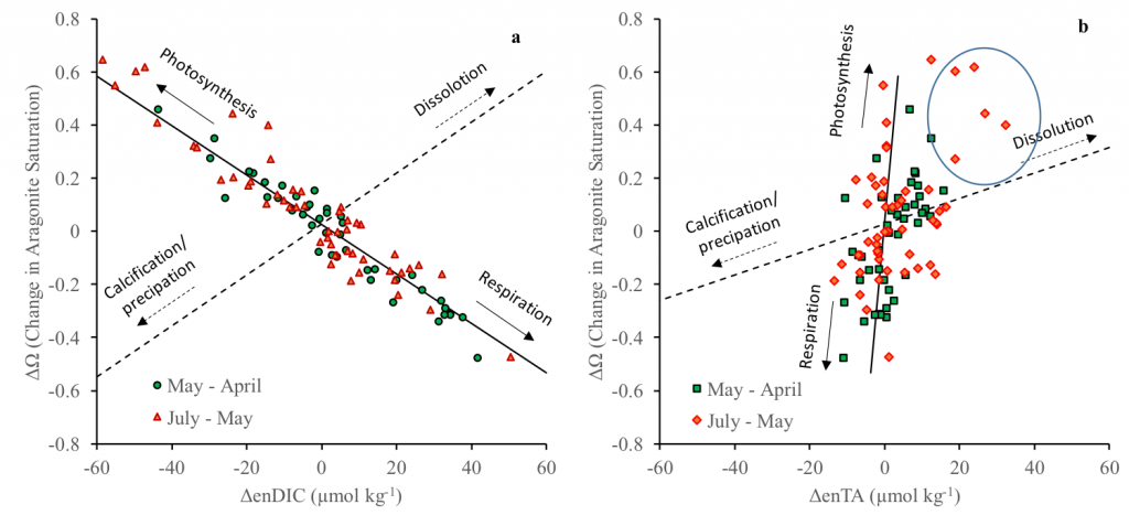
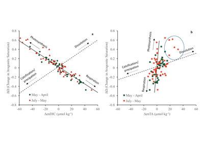
Figure. Changes of aragonite saturation states (ΔΩ) between three consecutive cruises from April – July 2015 as a function of changes in salinity-normalized DIC (ΔenDIC, including correction of freshwater inputs) (a) and changes in salinity-normalized TA (ΔenTA, including correction of freshwater inputs) (b). The data points circled in (b) represent potential alkalinity sources from CaCO3 dissolution and/or anaerobic respiration. Solid lines are theoretical lines of ΔΩ vs. ΔenDIC and ΔΩ vs. ΔenTA expected if only photosynthesis and respiration/remineralization occur. Dashed lines are theoretical lines if only calcification and dissolution of CaCO3 occur.
Under the current rate of OA, the mean Ω-Ar of the subsurface and bottom waters of the GoME will approach undersaturation (Ω-Ar < 1) in 30-40 years. As photosynthesis and respiration are the major driving mechanisms of Ω-Ar variability in the water column, any biological regime changes may significantly impact carbonate chemistry and the GoME ecosystem, including the CaCO3 shell-building capacity of organisms that are critical to the GoME food web.
Author:
Zhaohui Aleck Wang (Woods Hole Oceanographic Institution)