upwelling :: Ocean Carbon & Biogeochemistry

Studying marine ecosystems and biogeochemical cycles in the face of environmental change

Archive for upwelling

Turbulent Mixing: A Dominant Source of Oxygen in the Upper Equatorial Pacific

Posted by mmaheigan

· Tuesday, March 12th, 2024

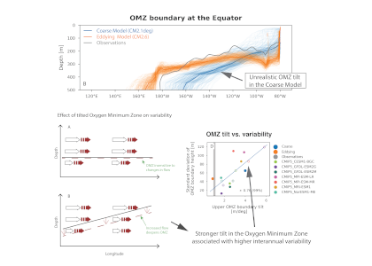
What balances oxygen removal in the equatorial Pacific? For a long time, oxygen in the eastern and central tropical Pacific was assumed to be mainly supplied by the large-scale advection of remotely ventilated waters via the equatorial current system and meridional circulation. A recent study used an eddy-resolving simulation of a global ocean model to show that turbulent mixing and its regulation by mesoscale eddies play a critical role in balancing oxygen removal (by consumption and upwelling) in the upper thermocline. Deeper in the water column, mean advection by the zonal currents and meridional circulation dominates. This mixing is tightly regulated by tropical instability waves, which intensify the shear between the equatorial currents and enhance the downward turbulent mixing flux of oxygen into the thermocline. Mesoscale phenomena thus play an indirect yet critical role as a local pathway of ventilation in this region. Testing these model-based hypotheses in the real ocean through dedicated field studies and long-term observations is needed to advance our understanding of the observed expansion of the oxygen deficient zones (ODZs) and model their future trajectory in a warmer and more stratified ocean.

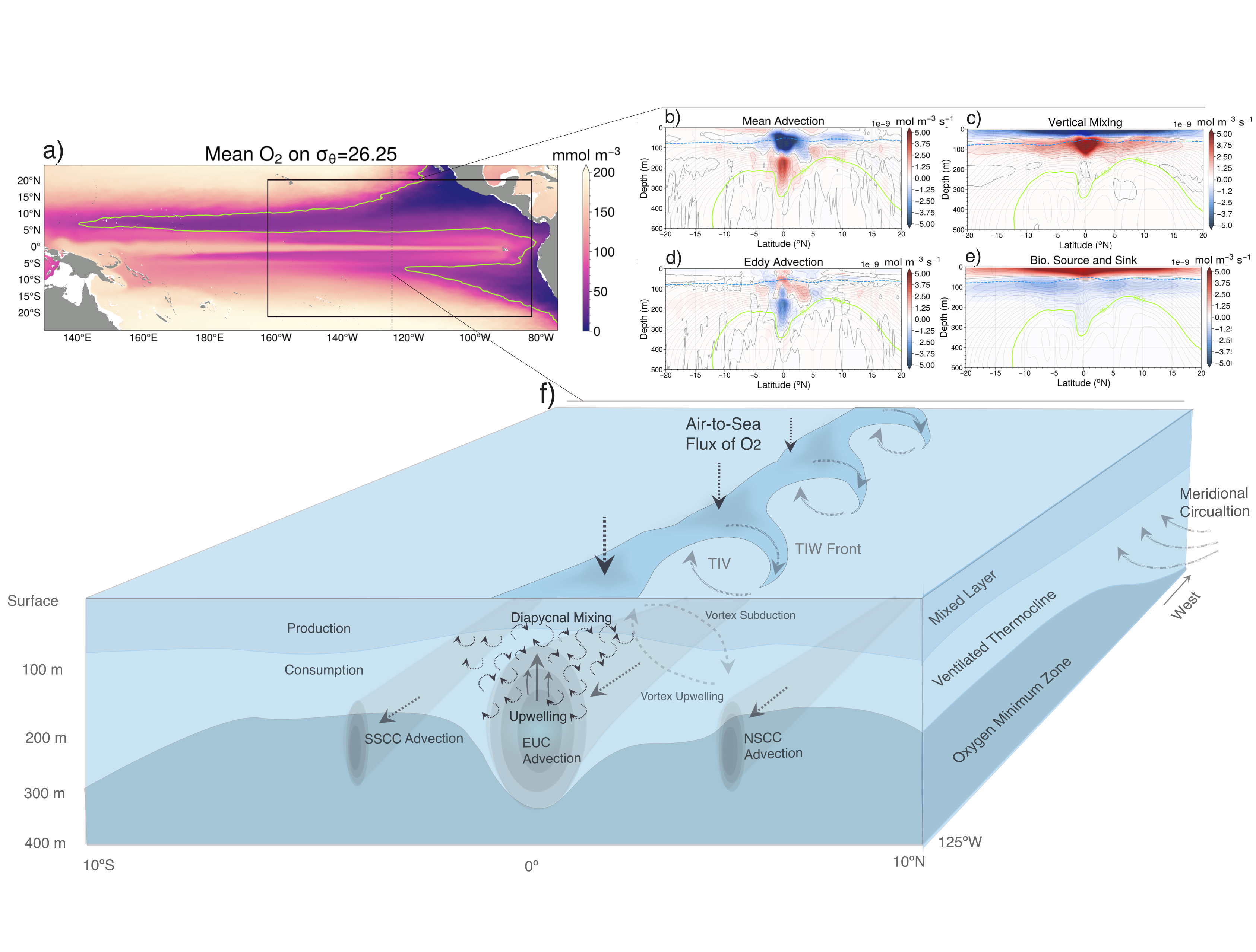
Figure: The main processes that set the mean structure of oxygen in the equatorial Pacific are assessed in an eddy resolving simulation of the Community Earth System Model (CESM). Panel a shows the climatological oxygen distribution on the 26.25 isopycnal in CESM. Panels b-e show the contribution of advection by mean circulation and eddies, vertical mixing, and production and consumption. These processes are illustrated in panel f). Figure adapted from Eddebbar et al (2024).

Authors
Yassir A. Eddebbar (Scripps Institution of Oceanography)
Daniel B. Whitt (NASA Ames)
Ariane Verdy, (Scripps Institution of Oceanography)
Matthew R. Mazloff (Scripps Institution of Oceanography)
Aneesh C. Subramanian (CU Boulder)
Matthew C. Long, (National Center for Atmospheric Research)

Air-sea gas disequilibrium drove deoxygenation of the deep ice-age ocean

Posted by mmaheigan

· Thursday, March 18th, 2021

During the Last Glacial Maximum (~20,000 years ago, LGM) sediment data show that the deep ocean had lower dissolved oxygen (O₂) concentrations than the preindustrial ocean, despite cooler temperatures of this period increasing O₂ solubility in sea water.

Figure 1. a) Whole ocean inventory of the O₂ components in the preindustrial control (PIC): total O₂ (O₂); the preformed components equilibrium O₂ (O₂ equilibrium), physical disequilibrium O₂ (O₂ diseq phys) and biologically-mediated disequilibrium (O₂ diseq bio); and O₂ respired from soft-tissue (O₂ soft). b) The difference in whole ocean inventory of O₂ components between the LGM and PIC simulations.

In a study published in Nature Geoscience, the authors provide one of the first explanations for glacial deoxygenation. The authors combined a data-constrained model of the preindustrial (PIC) and LGM ocean with a novel decomposition of O₂ to assess the processes affecting the oceanic distribution of oxygen. The decomposition allowed for the preformed disequilibrium O₂—the amount of oxygen that deviates from its solubility equilibrium value when at the surface—to be tracked, along with other contributions such as the O₂ consumed by bacterial respiration of organic matter. In the preindustrial ocean, a third of the subsurface oxygen deficit was a result of disequilibrium rather than oxygen consumed by bacteria. This contradicts previous assumptions (Figure 1a). Nearly 80% of the disequilibrium resulted from upwelling waters, depleted in O₂ due to respiration, not fully equilibrating before re-subduction into the ocean interior. This effect was even greater during the LGM (Figure 1b). The authors attributed this largely to the widespread presence of sea ice—which acts as a cap on the surface preventing the water from gaining oxygen from the atmosphere—in the ocean around Antarctica, with a smaller contribution from iron fertilization.

This study provides one of the first mechanistic explanations for LGM deep ocean deoxygenation. As the ocean is currently losing oxygen due to warming, the effect of other processes, including sea ice changes, could prove important for understanding long-term ocean oxygenation changes.

Authors
Ellen Cliff (University of Oxford)
Samar Khatiwala (University of Oxford)
Andreas Schmittner (Oregon State University)

Joint highlight with GEOTRACES International Project Office

The role of nutrient trapping in promoting shelf hypoxia in the southern Benguela upwelling system

Posted by mmaheigan

· Thursday, September 3rd, 2020

The southern Benguela upwelling system (SBUS) off southwest Africa is an exceptionally fertile ocean region that supports valuable commercial fisheries. The productivity of this system derives from the upwelling of nutrient-rich Subantarctic Mode Water, and from the concurrent entrainment of nutrients regenerated proximately on the expansive continental shelf. The SBUS is prone to severe seasonal hypoxic events that decimate regional fisheries, occurrences of which are inextricably linked to the inherent nutrient dynamics. In a study recently published in JGR Oceans, the authors sought to understand the mechanisms sustaining elevated concentrations and seasonally-variable distributions of nutrients in the SBUS, in relation to the subsurface oxygen content. Inter-seasonal measurements of nutrients and nitrate isotope ratios across the SBUS in 2017 revealed that upwards of 48% (summer) and 63% (winter) of the on‐shelf nutrients derived from regeneration in situ. The severity of hypoxia at the shelf bottom, in turn, correlated with the incidence of regenerated nutrients. The accrual of nutrients at the shelf bottom appears to be aided by hydrographic fronts that restrict offshore transport, trapping regenerated nutrients on the SBUS shelf and increasing the pool of nutrients available for upwelling – ultimately contributing to hypoxic events. This study underscores the need – if we are to develop a mechanistic and predictive understanding of hypoxia in the SBUS and elsewhere – to elucidate the role of shelf circulation in promoting the accrual of regenerated nutrients on the continental shelf. The next step is to combine new and existing observations with quantitative simulations to further interrogate the coupled physical-biogeochemical mechanisms that modulate the intensity of hypoxia.

Figure caption: Schematic of proposed nutrient-trapping mechanism: Deep nutrient-rich Subantarctic Mode Water (SAMW) acquires more nutrients as it passes over the shelf sediments from the regeneration of exported particulate organic material (POM). The production of this POM is fueled by nutrients stripped from the surface waters advecting back off-shore. The thickness of the arrows represents nutrient concentrations. Triangles indicate the positions of the Shelf Break Front (SBF) and Columbine Front (CF), coincident with an observed subduction of the Ekman layer and downwelling at the inner front boundary.

Authors
Raquel Flynn (University of Cape Town)
Julie Granger (University of Connecticut)
Jennifer Veitch (South African Environmental Observation Network)
Samantha Siedlecki (University of Connecticut)
Jessica Burger (University of Cape Town)
Keshnee Pillay (South Africa Department of Environment, Forestry and Fisheries)
Sarah Fawcett (University of Cape Town)

Multiyear predictions of ocean acidification in the California Current System

Posted by mmaheigan

· Thursday, August 20th, 2020

The California Current System is a highly productive coastal upwelling region that supports commercial fisheries valued at $6 billion/year. These fisheries are supported by upwelled waters, which are rich in nutrients and serve as a natural fertilizer for phytoplankton. Due to remineralization of organic matter at depth, these upwelled waters also contain large amounts of dissolved inorganic carbon, causing local conditions to be more acidic than the open ocean. This natural acidity, compounded by the dissolution of anthropogenic CO₂ into coastal waters, creates corrosive conditions for shell-forming organisms, including commercial fishery species.

A recent study in Nature Communications showcases the potential for climate models to skillfully predict variations in surface pH—thus ocean acidification—in the California Current System. The authors evaluate retrospective predictions of ocean acidity made by a global Earth System Model set up similarly to a weather forecasting system. The forecasting system can already predict variations in observed surface pH fourteen months in advance, but has the potential to predict surface pH up to five years in advance with better initializations of dissolved inorganic carbon (Figure 1). Skillful predictions are mostly driven by the model’s initialization and subsequent transport of dissolved inorganic carbon throughout the North Pacific basin.

Figure 1. Forecast of annual surface pH anomalies in the California Current Large Marine Ecosystem for 2020. Red colors denote anomalously basic conditions for the given location and blue colors indicate anomalously acidic conditions.

These results demonstrate, for the first time, the feasibility of using climate models to make multiyear predictions of surface pH in the California Current. Output from this global prediction system could serve as boundary conditions for high-resolution models of the California Current to improve prediction time scale and ultimately help inform management decisions for vulnerable and valuable shellfisheries.

Authors:
Riley X. Brady (University of Colorado Boulder)
Nicole S. Lovenduski (University of Colorado Boulder)
Stephen G. Yeager (National Center for Atmospheric Research)
Matthew C. Long (National Center for Atmospheric Research)
Keith Lindsay (National Center for Atmospheric Research)

Physics vs. biology in Southern Ocean nutrient gradients

Posted by mmaheigan

· Tuesday, June 16th, 2020

In the Southern Ocean, surface water silicate (SiO₄) concentrations decline very quickly relative to nitrate concentrations along a northward gradient toward mode water formation regions on the northern edge (Figure 1a, b). These mode waters play a critical role in driving global nutrient concentrations, setting the biogeochemistry of low- and mid-latitude regions around the globe after they upwell further north. To explain this latitudinal surface gradient, most hypotheses have implicated diatoms, which take up and export silicon as well as nitrogen: (1) Diatoms, including highly-silicified species such as Fragilariopsis kerguelensis, are more abundant in the Southern Ocean than elsewhere; (2) Iron limitation, which is prevalent in the Southern Ocean, elevates the Si:N ratio of diatoms; (3) Mass export of empty diatom frustules pumps silicate but not nitrate to deeper waters.

Figure 1: (a) and (b) nitrate and silicate concentrations in surface waters of the Southern Ocean (GLODAPv2_2019 data). (c) Model results of a standard run (black diamonds), a run without biology (red diamonds) and a run without mixing (blue diamonds).

In a recent paper published in Biogeosciences, the authors use an idealized model to explore the relative roles of biological vs. physical processes in driving the observed latitudinal surface nutrient gradients. Over timescales of a few years, removing the effects of biology (no SiO₄uptake or export) from the model elevates silicate concentrations slightly over the entire latitudinal range, but does not remove the strong latitudinal gradient (Figure 1c). However, if the effects of vertical mixing processes such as upwelling and entrainment are removed from the model by eliminating the observed deep [SiO₄] gradient, the observed surface nutrient gradient is greatly altered (Figure 1c). These model results suggest that, over short timescales, physics is more important than biology in driving the observed surface water gradient in SiO₄:NO₃ ratios and forcing silicate depletion of mode waters leaving the Southern Ocean. These findings add to our understanding of Southern Ocean dynamics and the downstream effects on other oceans.

Authors:
P. Demuynck (University of Southampton)
T. Tyrrell (University of Southampton)
A.C. Naveira Garabato (University of Southampton)
C.M. Moore (University of Southampton)
A.P. Martin (National Oceanography Centre)

The Equatorial Undercurrent influences the fate of the Oxygen Minimum Zone in the Pacific

Posted by mmaheigan

· Tuesday, November 12th, 2019

While the ocean as a whole is losing oxygen due to warming, oxygen minimum zones (OMZs) are maintained by a delicate balance of biological and physical processes; it is unclear how each one of them is going to evolve in the future. Changes to OMZs could affect the global uptake of carbon, the generation of greenhouse gases, and interactions among marine life. Current generation coarse-resolution (~1°) climate models compromise the ability to simulate low-oxygen waters and their response to climate change in the future because they fail to reproduce a major ocean current, the Equatorial Undercurrent (EUC). These shortcomings lead to an overly tilted upper oxygen minimum zone (OMZ) (Figure 1), thus exaggerating sensitivity to circulation changes and overwhelming other key processes like diffusion and biology. The EUC also plays a vital role in feeding the eastern Pacific upwelling region, connecting it to global climate variability.

Figure: Top: The boundary of the Oxygen Minimum Zone (OMZ) along the Equator is unrealistically tilted for current generation (coarse resolution) climate models, and improves with increased horizontal resolution. The tilt is due to a bad representation of the Equatorial Undercurrent in the coarse model, also seen in other coarse models. The exaggerated tilt of the OMZ boundary at the Equator leads to increased inter-annual variability of the depth of the upper OMZ boundary, via changes in the zonal flow (left). This phenomenon is found in most CMIP5 models (right) and could be responsible for the current inability to predict the change in OMZ extent for the next century.

A recent high‐resolution climate model study in Geophysical Research Letters significantly improved the representation of both the EUC and OMZ, suggesting that the EUC is a key player in OMZ variability. This study emphasizes the importance of improving transport processes in global circulation models to better simulate oxygen distribution and predict future OMZ extent. The results of this study imply that the fundamental dynamics maintaining this key ocean current could be categorically misrepresented in the current generation of climate models, potentially influencing the ability to predict future climate variability and trends.

Authors:
Julius J.M. Busecke (Princeton University)
Laure Resplandy (Princeton University)
John P. Dunne (NOAA/GFDL)

Arctic surface waters release methane but also absorb 2,000 times the CO2 for a net cooling effect

Posted by mmaheigan

· Thursday, September 28th, 2017

A recent study by Pohlman et al. published in PNAS showed that ocean waters near the surface of the Arctic Ocean absorbed 2,000 times more carbon dioxide (CO₂) from the atmosphere than the amount of methane released into the atmosphere from the same waters. The study was conducted near Norway’s Svalbard Islands, which overly numerous seafloor methane seeps.

Methane is a more potent greenhouse gas than CO₂, but the removal of CO₂from the atmosphere where the study was conducted more than offset the potential warming effect of the observed methane emissions. During the study, scientists continuously measured the concentrations of methane and CO₂ in near-surface waters and in the air just above the ocean surface. The measurements were taken over methane seeps fields at water depths ranging from 260 to 8530 feet (80 to 2600 meters).

Figure 1. Ocean waters overlying shallow-water methane seeps (white dots) offshore from the Svalbard Islands absorb substantially more atmospheric carbon dioxide than the methane that they emit to the atmosphere. Colors indicate the strength of the negative greenhouse warming potential associated with carbon dioxide influx to these surface waters relative to the positive greenhouse warming potential associated with the methane emissions. Gray shiptracks have background values for the relative greenhouse warming potential.

Analysis of the data confirmed that methane was entering the atmosphere above the shallowest (water depth of 260-295 feet or 80-90 meters) Svalbard margin seeps. The data also showed that significant amounts of CO₂ were being absorbed by the waters near the ocean surface, and that the cooling effect resulting from CO₂ uptake is up to 230 times greater than the warming effect expected from the methane emitted.

Most previous studies have focused only on the sea-air flux of methane overlying seafloor seep sites and have not accounted for the drawdown of CO₂that could offset some of the atmospheric warming potential of the methane. Phytoplankton appeared to be more active in the near-surface waters overlying the seafloor methane seeps, which would explain why so much carbon dioxide was being absorbed. Physical and biogeochemical measurements of near-surface waters overlying the seafloor methane seeps showed strong evidence of upwelling of cold, nutrient-rich waters from depth, stimulating phytoplankton activity and increasing CO₂ drawdown. This study was the first to document this CO₂ drawdown mechanism in a methane source region.

“If what we observed near Svalbard occurs more broadly at similar locations around the world, it could mean that methane seeps have a net cooling effect on climate, not a warming effect as we previously thought,” said USGS biogeochemist John Pohlman, the paper’s lead author. “We are looking forward to testing the hypothesis that shallow-water methane seeps are net greenhouse gas sinks in other locations.”

Authors:
John W. Pohlman (USGS Woods Hole Coastal & Marine Science Center)
Jens Greinert (GEOMAR, Univ. of Tromsø, Royal Netherlands Institute for Sea Research)
Carolyn Ruppel (USGS Woods Hole Coastal & Marine Science Center)
Anna Silyakova (Univ. of Tromsø)
Lisa Vielstädte (GEOMAR)
Michael Casso (USGS Woods Hole Coastal & Marine Science Center)
Jürgen Mienert (Univ. of Tromsø)
Stefan Bünz (Univ. of Tromsø)

Untangling the mystery of domoic acid events: A climate-scale perspective

Posted by mmaheigan

· Thursday, August 3rd, 2017

The diatom Pseudo-nitzchia produces a neurotoxin called domoic acid, which in high concentrations affects wildlife ranging from mussels and crabs to seabirds and sea lions, as well as humans. In humans, the effects of domoic acid poisoning can range from gastrointestinal distress to memory loss, and even death. Despite being studied in laboratories since the late 1980s, there is no consensus on the environmental conditions that lead to domoic acid events. These events are most frequent and impactful in eastern boundary current regions such as the California Current System, which is bordered by Washington, Oregon, and California. In Oregon alone, there have been six major domoic acid events: 1996, 1998-1999, 2001, 2002-2006, 2010, 2014-2015. McKibben et al. (2017) investigated the regulation of domoic acid at a climate scale to develop and test an applied risk model for the US West Coast” to read “McKibben et al. (2017) investigated the regulation of domoic acid at regional and decadal scales in order to develop and test an applied risk model for the impact of climate on the US West Coast. They used the PDO and ONI climate variability indices, averages of monthly and 3 month running means of SST anomaly values and variability to look at basin-scale ocean conditions. At a local scale, data were from zooplankton sampling every two to four weeks between 1996 to 2015 at hydrographic station offshore of Newport, OR. Additionally, the NOAA NCDC product “Daily Optimum Interpolation, Advanced Very High Resolution Radiometer Only, Version 2, Final+Preliminary SST” was used to obtain the monthly SST anomaly metric, based on combined in situ and satellite data.

(A) Warm and cool ocean regimes, (B) local SST anomaly, and (C and D) biological response. (A) PDO (red or blue vertical bars) and ONI (black line) indices; strong (S) to moderate (M) El Nino (+1) and La Nina (−1) events are labeled. (B) SST anomaly 20 nm off central OR. (C) The CSR anomaly 5 nm off central OR. (D) Monthly OR coastal maximum DA levels in razor clams (vertical bars); horizontal black line is the 20-ppm closure threshold. Black line in D shows the spring biological transition date (right y axis). At the top of the figure, black boxes indicate the duration of upwelling season each year; red vertical bars indicate the timing of annual DA maxima in relationship to upwelling. Gray shaded regions are warm regimes based on the PDO. Dashed vertical lines indicate onset of the six major DA events. The September 2014 arrival of the NE Pacific Warm Anomaly (colloquially termed “The Blob”) to the OR coastal region is labeled on B. “X” symbols along the x axes indicate that no data were available for that month (B–D).

Their findings show that these events have occurred when there is advection of warmer water masses onto the continental shelf from southern or offshore areas. When the warm phase of the Pacific Decadal Oscillation (PDO) and El Niño coincide, the effect is additive. In the warm regime years, there is a later spring biological transition date, weaker alongshore currents, elevated water temperatures, and plankton communities are dominated by subtropical rather than subarctic species. The authors also note relative differences between the prevalence and phenology of domoic acid events in OR, CA and WA, which warrants further study via regional-scale modeling. Overall, this research shows a clear and enhanced risk of toxicity in shellfish during warm phases of natural climate oscillations. If predictions of more extreme warming come to bear, this would potentially lead to increased DA event intensity and frequency in coastal zones around the globe. This will not only affect wildlife, but may cause significant closures of economically important fisheries (e.g., Dungeness crab, anchovy, mussel, and razor clam), which would impact local communities and native populations.

Authors:
Morgaine McKibben (Oregon State Univ., NOAA Northwest Fisheries Science Center)
William Peterson (NOAA Northwest Fisheries Science Center)
Michelle Wood (Univ. Oregon)
Vera L. Trainer (NOAA Northwest Fisheries Science Center)
Matthew Hunter (Oregon Dept. Fish & Wildlife)
Angelicque E. White (Oregon State Univ.)

A framework for ENSO predictability of marine ecosystem drivers along the US West Coast

Posted by mmaheigan

· Thursday, February 16th, 2017

The US West Coast eastern boundary upwelling system supports one of the most productive marine ecosystems in the world and is a primary source of ecosystem services for the US (e.g., fishing, shipping, and recreation). Long-term historical observations of physical and biological variables in this region have been collected since the 1950s (e.g., the CalCOFI program and now including the coastal ocean observing systems), leading to an excellent foundation for understanding the ecosystem impacts of dominant climate fluctuations such as the El Niño-Southern Oscillation (ENSO). In the northeast Pacific, ENSO impacts a wide range of physical and biotic processes, including temperature, stratification, winds, upwelling, and primary and secondary production. The El Niño phase of ENSO, in particular, can result in extensive geographic habitat range displacements and altered catches of fishes and invertebrates, and impact vertical and lateral export fluxes of carbon and other elements (Jacox et al., this issue; Anderson et al., this issue; Ohman et al., this issue). However, despite empirical observations and increased understanding of the coupling between climate and marine ecosystems along the US West Coast, there has been no systematic attempt to use this knowledge to forecast marine ecosystem responses to individual ENSO events. ENSO forecasting has become routine in the climate community. However, little has been done to forecast the impacts of ENSO on ecosystems and their services. This becomes especially important considering the occurrence of recent strong El Niño events (such as 2015-16) and climate model projections that suggest that ENSO extremes may become more frequent (Cai et al. 2015).

The joint US CLIVAR/OCB/NOAA/PICES/ICES workshop on Forecasting ENSO impacts on marine ecosystems of the US West Coast (Di Lorenzo et al. 2017) held in La Jolla, California, in August 2016 outlined a three-step strategy to better understand and quantify the ENSO-related predictability of marine ecosystem drivers along the US West Coast (Figure 1). The first step is to use a high-resolution ocean reanalysis to determine the association between local ecosystem drivers and regional forcing patterns (RFPs). The identification of ecosystem drivers will depend on the ecosystem indicators or target species selected for prediction (Ohman et al., this issue). The second step is to objectively identify the tropical sea surface temperature (SST) patterns that optimally force the RFPs along the US West Coast region using available long-term large-scale reanalysis products. While the goal of the first two steps is to understand the dynamical basis for predictability (Figure 1, blue path), the final third step (Figure 1, orange path) aims at quantifying the predictability of the RFPs and estimating their prediction skill at seasonal timescales. This third step can be implemented using the output of multi-model ensemble forecasts such as the North America Multi-Model Ensemble (NMME) or by building efficient statistical prediction models such as Linear Inverse Models (LIMs; Newman et al. 2003).

Figure 1. Framework for understanding and predicting ENSO impacts on ecosystem drivers. Blue path shows the steps that will lead to Understanding of the ecosystem drivers and their dependence on tropical Pacific anomalies. Orange path shows the steps that will lead to quantifying the Predictability of marine ecosystem drivers along the US West Coast that are predictable from large-scale tropical teleconnection dynamics.

Important to the concept of ENSO predictability is the realization that the expressions of ENSO are very diverse and cannot be identified with a few indices (Capotondi et al. 2015; Capotondi et al., this issue). In fact, different expressions of sea surface temperature anomalies (SSTa) in the tropics give rise to oceanic and atmospheric teleconnections that generate different coastal impacts in the northeast Pacific. For this reason, we will refer to ENSO as the collection of tropical Pacific SSTa that lead to deterministic and predictable responses in the regional ocean and atmosphere along the US West Coast.

In the sections below, we articulate in more detail the elements of the framework for quantifying the predictability of ENSO-related impacts on coastal ecosystems along the US West Coast (Figure 1). Our focus will be on the California Current System (CCS), reflecting the regional expertise of the workshop participants. Specifically, we discuss (1) the ecosystem drivers and what is identified as such; (2) RFP definitions; and (3) the teleconnections from the tropical Pacific and their predictability.

Ecosystem drivers in the California Current System

The impacts of oceanic processes on the CCS marine ecosystem have been investigated since the 1950s when the long-term California Cooperative Oceanic Fisheries Investigations (CalCOFI) began routine seasonal sampling of coastal ocean waters. The CalCOFI program continues today and has been augmented with several other sampling programs (e.g., the coastal ocean observing network), leading to an unprecedented understanding of how climate and physical ocean processes, such as upwelling, drive ecosystem variability and change (e.g., see more recent reviews from King et al.2011; Ohman et al. 2013; Di Lorenzo et al. 2013).

The dominant physical oceanographic drivers of ecosystem variability occur on seasonal, interannual, and decadal timescales and are associated with changes in (1) SST; (2) upwelling velocity; (3) alongshore transport; (4) cross-shore transport; and (5) thermocline/nutricline depth (see Ohman et al., this issue). This set of ecosystem drivers emerged from discussions among experts at the workshop. Ecosystem responses to these drivers include multiple trophic levels, including phytoplankton, zooplankton, small pelagic fish, and top predators, and several examples have been identified for the CCS (see summary table in Ohman et al., this issue).

While much research has focused on diagnosing the mechanisms by which these physical drivers impact marine ecosystems, less is known about the dynamics controlling the predictability of these drivers. As highlighted in Ohman et al. (this issue), most of the regional oceanographic drivers (e.g., changes in local SST, upwelling, transport, thermocline depth) are connected to changes in large-scale forcings (e.g., winds, surface heat fluxes, large-scale SST and sea surface height patterns, freshwater fluxes, and remotely forced coastally trapped waves entering the CCS from the south). In fact, several studies have documented how large-scale changes in wind patterns associated with the Aleutian Low and the North Pacific Oscillation drive oceanic modes of variability such as the Pacific Decadal Oscillation and the North Pacific Gyre Oscillation (Mantua et al. 1997; Di Lorenzo et al. 2008; Chhak et al. 2009; Ohman et al., this issue; Jacox et al., this issue; Anderson et al., this issue; Capotondi et al., this issue) that influence the CCS. However, these large-scale modes only explain a fraction of the ecosystem’s atmospheric forcing functions at the regional-scale. Thus, it is important to identify other key forcings to gain a more complete mechanistic understanding of CCS ecosystem drivers (e.g., Jacox et al. 2014; 2015).

Atmospheric and oceanic regional forcing patterns

The dominant large-scale quantities that control the CCS ecosystem drivers are winds, heat fluxes, and remotely forced coastally trapped waves (Hickey 1979). Regional expressions or patterns of these large-scale forcings have been linked to changes in local stratification and thermocline depth (Veneziani et al. 2009a; 2009b; Combes et al. 2013), cross-shore transport associated with mesoscale eddies (Kurian et al. 2011; Todd et al. 2012; Song et al. 2012; Davis and Di Lorenzo 2015b), and along-shore transport (Davis and Di Lorenzo 2015a; Bograd et al. 2015). For this reason, we define the regional expressions of the atmospheric and remote wave forcing that are optimal in driving SST, ocean transport, upwelling, and thermocline depth as the RFPs. To clarify this concept, consider the estimation of coastal upwelling velocities. While a change in the position and strength in the Aleutian Low has been related to coastal upwelling in the northern CCS, a more targeted measure of the actual upwelling vertical velocity and nutrient fluxes that are relevant to primary productivity can only be quantified by taking into account a combination of oceanic processes that depend on multiple RFPs such as thermocline depth (e.g., remote waves), thermal stratification (e.g., heat fluxes), mesoscale eddies, and upwelling velocities (e.g., local patterns of wind stress curl and alongshore winds; see Gruber et al 2011; Jacox et al. 2015; Renault et al. 2016). In other words, if we consider the vertical coastal upwelling velocity (w) along the northern CCS, a more adequate physical description and quantification would be given from a linear combination of the different regional forcing functions w = Σ_n∝_n * RFP_n rather than w = ∝*Aleutian Low.

The largest interannual variability in the Pacific that impacts the RFPs is ENSO, which also constitutes the largest source of seasonal (3-6 months) predictability. During El Niño and La Niña, atmospheric and oceanic teleconnections from the tropics modify large-scale and local surface wind patterns and ocean currents of the CCS and force coastally trapped waves.

ENSO teleconnections and potential seasonal predictability of the regional forcing patterns

While ENSO exerts important controls on the RFPs in the CCS, it has become evident that ENSO expressions in the tropics vary significantly from event to event, leading to different responses in the CCS (Capotondi et al., this issue). Also, as previously pointed out, the CCS is not only sensitive to strong ENSO events but more generally responds to a wide range of tropical SSTa variability that is driven by ENSO-type dynamics in the tropical and sub-tropical Pacific. For this reason, we define an “ENSO teleconnection” as any RFP response that is linked to ENSO-type variability in the tropics.

ENSO can influence the upwelling and circulation in the CCS region through both oceanic and atmospheric pathways. It is well known that equatorial Kelvin waves, an integral part of ENSO dynamics, propagate eastward along the Equator and continue both northward (and southward) along the coasts of the Americas as coastally trapped Kelvin waves after reaching the eastern ocean boundary. El Niño events are associated with downwelling Kelvin waves, leading to a deepening of the thermocline, while La Niña events produce a shoaling of the thermocline in the CCS (Simpson 1984; Lynn and Bograd 2002; Huyer et al. 2002; Bograd et al. 2009; Hermann et al. 2009; Miller et al. 2015). The offshore scale of coastal Kelvin waves decreases with latitude, and the waves decay while propagating northward along the coast due to dissipation and radiation of westward propagating Rossby waves. In addition, topography and bathymetry can modify the nature of the waves and perhaps partially impede their propagation at some location. Thus, the efficiency of coastal waves of equatorial origin in modifying the stratification in the CCS is still a matter of debate. To complicate matters, regional wind variability south of the CCS also excites coastally trapped waves, which supplement the tropical source.

In the tropics, SST anomalies associated with ENSO change tropical convection and excite mid-troposphere stationary atmospheric Rossby waves that propagate signals to the extratropics, the so-called atmospheric ENSO teleconnections (Capotondi et al., this issue). Through these atmospheric waves, warm ENSO events favor a deepening and southward shift of the Aleutian Low pressure system that is dominant during winter, as well as changes in the North Pacific Subtropical High that is dominant during spring and summer, resulting in a weakening of the alongshore winds, reduced upwelling, and warmer surface water. These changes are similar to those induced by coastal Kelvin waves of equatorial origin, making it very difficult to distinguish the relative importance of the oceanic and atmospheric pathways in the CCS. In addition, due to internal atmospheric noise, the details of the ENSO teleconnections can vary significantly from event to event and result in important differences along the California Coast (Figure 2).

Figure 2. Schematic of ENSO teleconnection associated with different flavors of tropical SSTa. (a) Atmospheric teleconnections of the canonical eastern Pacific El Niño tend to impact the winter expression of the Aleutian Low, which in turn drives an oceanic SSTa anomaly that projects onto the pattern of the Pacific Decadal Oscillation (PDO). (b) Atmospheric teleconnections of the central Pacific El Niño tend to impact the winter expression of the North Pacific High, which in turn drives an oceanic SSTa anomaly that projects onto the pattern of the North Pacific Gyre Oscillation (NPGO). The ENSO SSTa maps are obtained by regressing indices of central and eastern Pacific ENSO with SSTa. The other maps are obtained by regression of SSTa/SLPa with the PDO (a) and NPGO (b) indices.

El Niño events exhibit a large diversity in amplitude, duration, and spatial pattern (Capotondi et al. 2015). The amplitude and location of the maximum SST anomalies, whether in the eastern (EP) or central (CP) Pacific, can have a large impact on ENSO teleconnections (Ashok et al. 2007; Larkin and Harrison 2005). While “canonical” EP events induce changes in the Aleutian Low (Figure 2b), CP events have been associated with a strengthening of the second mode of North Pacific atmospheric variability, the North Pacific Oscillation (NPO; Figure 2a; Di Lorenzo et al. 2010; Furtado et al. 2012). In addition, it is conceivable that EP events have a larger Kelvin wave signature than CP events, resulting in different oceanic influences in the CCS.

In summary, while the ENSO influence on the CCS physical and biological environments is undeniable, several sources of uncertainty remain about the details of that influence. This uncertainty arises in the physical environment on seasonal timescales from many sources, including the diversity of ENSO events, the intrinsic unpredictable components of the atmosphere, and the intrinsic unpredictable eddy variations in the CCS. We also need to distinguish between physically forced ecosystem response versus intrinsic biological variability, which is potentially nonlinear and likely unpredictable. Skill levels need to be quantified for each step of the prediction process (i.e., ENSO, teleconnections, local oceanic response, local ecosystem response) relative to a baseline—for example the persistence of initial condition, which is also being exploited for skillful predictions of the large marine ecosystem at the seasonal timescale (Tommasi et al., this issue). The target populations should be exploitable species that are of interest to federal and state agencies that regulate certain stocks. Models are currently being developed to use ocean forecasts to advance top predator management (Hazen et al., this issue). The implementation of this framework (Figure 1) for practical uses will require a collaborative effort between physical climate scientists with expertise in predicting and understanding ENSO and biologists who have expertise in understanding ecosystem response to physical climate forcing.

Authors

Emanuele Di Lorenzo (Georgia Institute of Technology)
Arthur J. Miller (Scripps Institution of Oceanography)

References

Ashok, K., S.K. Behera, S.A. Rao, H. Weng, and T. Yamagata, 2007: El Niño Modoki and its possible teleconnections. J. Geophys. Res., 112, doi:10.1029/2006JC003798

Bograd, S. J., M. Pozo Buil, E. Di Lorenzo, C. G. Castro, I. D. Schroeder, R. Goericke, C. R. Anderson, C. Benitez-Nelson, and F. A. Whitney, 2015: Changes in source waters to the Southern California Bight. Deep-Sea Res. Part II-Top. Stud. Oceanogr., 112, 42-52, doi:10.1016/j.dsr2.2014.04.009.

Bograd, S. J., I. Schroeder, N. Sarkar, X. Qiu, W. J. Sydeman, and F. B. Schwing, 2009: Phenology of coastal upwelling in the California Current. Geophy. Res. Lett., 36, doi: 10.1029/2008GL035933.

Cai, W. J., and Coauthors, 2015: ENSO and greenhouse warming. Nature Climate Change, 5, 849-859, doi:10.1038/nclimate2743.

Capotondi, A., and Coauthors, 2015: Understanding ENSO Diversity. Bull. Amer. Meteor. Soc., 96, 921-938, doi:10.1175/BAMS-D-13-00117.1.

Chhak, K. C., E. Di Lorenzo, N. Schneider, and P. F. Cummins, 2009: Forcing of low-frequency ocean variability in the northeast Pacific. J. Climate, 22, 1255-1276, doi:10.1175/2008jcli2639.1.

Davis, A., and E. Di Lorenzo, 2015a: Interannual forcing mechanisms of California Current transports I: Meridional Currents. Deep-Sea Res. Part II-Top. Stud. Oceanogr., 112, 18-30, doi:10.1016/j.dsr2.2014.02.005.

Davis, A., and E. Di Lorenzo, 2015b: Interannual forcing mechanisms of California Current transports II: Mesoscale eddies. Deep-Sea Res. Part II-Top. Stud. Oceanogr., 112, 31-41, doi:10.1016/j.dsr2.2014.02.004.

Di Lorenzo, E., and Coauthors, 2017: Forecasting ENSO impacts on marine ecosystems of the US West Coast, Joint US CLIVAR/NOAA/PICES/ICES Report, https://usclivar.org/meetings/2016-enso-ecosystems, forthcoming.

Di Lorenzo, E., and Coauthors, 2008: North Pacific Gyre Oscillation links ocean climate and ecosystem change. Geophys. Res. Lett., 35, doi:10.1029/2007gl032838.

Di Lorenzo, E., and Coauthors, 2013: Synthesis of Pacific Ocean climate and ecosystem dynamics. Oceanogr., 26, 68-81, doi: 10.5670/oceanog.2013.76.

Di Lorenzo, E., K. M. Cobb, J. C. Furtado, N. Schneider, B. T. Anderson, A. Bracco, M. A. Alexander, and D. J. Vimont, 2010: Central Pacific El Nino and decadal climate change in the North Pacific Ocean. Nature Geosci., 3, 762-765, doi:10.1038/ngeo984.

Furtado, J. C., E. Di Lorenzo, B. T. Anderson, and N. Schneider, 2012: Linkages between the North Pacific Oscillation and central tropical Pacific SSTs at low frequencies. Climate Dyn., 39, 2833-2846, doi:10.1007/s00382-011-1245-4.

Gruber, N., Z. Lachkar, H. Frenzel, P. Marchesiello, M. Munnich, J. C. McWilliams, T. Nagai, and G. K. Plattner, 2011: Eddy-induced reduction of biological production in eastern boundary upwelling systems. Nature Geosci., 4, 787-792, doi:10.1038/ngeo1273.

Hermann, A. J., E. N. Curchitser, D. B. Haidvogel, and E. L. Dobbins, 2009: A comparison of remote vs. local influence of El Nino on the coastal circulation of the northeast Pacific. Deep Sea Res. Part II: Top. Stud. Oceanogr., 56, 2427-2443, doi: 10.1016/j.dsr2.2009.02.005.

Hickey, B. M., 1979. The California Current system—hypotheses and facts. Prog. Oceanogr., 8, 191-279, doi: 10.1016/0079-6611(79)90002-8.

Huyer, A., R. L. Smith, and J. Fleischbein, 2002: The coastal ocean off Oregon and northern California during the 1997–8 El Nino. Prog. Oceanogr., 54, 311-341, doi: 10.1016/S0079-6611(02)00056-3.

Jacox, M. G., A. M. Moore, C. A. Edwards, and J. Fiechter, 2014: Spatially resolved upwelling in the California Current System and its connections to climate variability. Geophy. Res. Lett., 41, 3189-3196, doi:10.1002/2014gl059589.

Jacox, M. G., J. Fiechter, A. M. Moore, and C. A. Edwards, 2015: ENSO and the California Current coastal upwelling response. J. Geophy. Res.-Oceans, 120, 1691-1702, doi:10.1002/2014jc010650.

Jacox, M. G., S. J. Bograd, E. L. Hazen, and J. Fiechter, 2015: Sensitivity of the California Current nutrient supply to wind, heat, and remote ocean forcing. Geophys. Res. Lett., 42, 5950-5957, doi:10.1002/2015GL065147.

Jacox, M. G., E. L. Hazen, K. D. Zaba, D. L. Rudnick, C. A. Edwards, A. M. Moore, and S. J. Bograd, 2016: Impacts of the 2015-2016 El Niño on the California Current System: Early assessment and comparison to past events. Geophys. Res. Lett., 43, 7072-7080, doi:10.1002/2016GL069716.

King, J. R., V. N. Agostini, C. J. Harvey, G. A. McFarlane, M. G. G. Foreman, J. E. Overland, E. Di Lorenzo, N. A. Bond, and K. Y. Aydin, 2011: Climate forcing and the California Current ecosystem. Ices J. Mar. Sci., 68, 1199-1216, doi:10.1093/icesjms/fsr009.

Kurian, J., F. Colas, X. Capet, J. C. McWilliams, and D. B. Chelton, 2011: Eddy properties in the California Current System. J. Geophy. Res.-Oceans, 116, doi:10.1029/2010jc006895.

Larkin, N. K. and D. E. Harrison, 2005: On the definition of El Niño and associated seasonal average US weather anomalies. Geophy. Res. Lett. 32, doi: 10.1029/2005GL022738.

Lynn, R. J. and S. J. Bograd, 2002: Dynamic evolution of the 1997–1999 El Niño–La Niña cycle in the southern California Current system. Prog. Oceanogr., 54, 59-75, doi: 10.1016/S0079-6611(02)00043-5.

Mantua, N. J., S. R. Hare, Y. Zhang, J. M. Wallace, and R. C. Francis, 1997: A Pacific interdecadal climate oscillation with impacts on salmon production. Bull. Amer. Meteorol. Soc., 78, 1069-1079, doi:10.1175/1520-0477(1997)078<1069:apicow>2.0.co;2.

Marchesiello, P., J. C. McWilliams, and A. Shchepetkin, 2003: Equilibrium structure and dynamics of the California Current System. J. Phys. Oceanogr., 33, 753-783, doi: 10.1175/1520-0485(2003)33<753:ESADOT>2.0.CO;2.

McCreary, J. P., P. K. Kundu, and S. Y. Chao, 1987: On the dynamics of the California Current System. J. Mar. Res., 45, 1-32, doi: 10.1357/002224087788400945.

Miller, A. J., H. Song, and A. C. Subramanian, 2015: The physical oceanographic environment during the CCE-LTER Years: Changes in climate and concepts. Deep Sea Res. Part II: Top. Stud. Oceanogr., 112, 6-17, doi: 10.1016/j.dsr2.2014.01.003.

Newman, M., and Coauthors, 2016: The Pacific Decadal Oscillation, Revisited. J. Climate, 29, 4399-4427, doi:10.1175/jcli-d-15-0508.1.

Ohman, M. D., K. Barbeau, P. J. S. Franks, R. Goericke, M. R. Landry, and A. J. Miller, 2013: Ecological transitions in a coastal upwelling ecosystem. Oceanogr., 26, 210-219, doi: 10.5670/oceanog.2013.65.

Renault, L., C. Deutsch, J. C. McWilliams, H. Frenzel, J.-H. Liang, and F. Colas, 2016: Partial decoupling of primary productivity from upwelling in the California Current system. Nature Geosci, 9, 505-508, doi:10.1038/ngeo2722.

Simpson, J. J., 1984; El Nino‐induced onshore transport in the California Current during 1982‐1983. Geophy. Res. Lett., 11, 233-236, doi: 10.1029/GL011i003p00233.

Song, H., A. J. Miller, B. D. Cornuelle, and E. Di Lorenzo, 2011: Changes in upwelling and its water sources in the California Current System driven by different wind forcing. Dyn. Atmos. Oceans, 52, 170-191, doi:10.1016/j.dynatmoce.2011.03.001.

Todd, R. E., D. L. Rudnick, M. R. Mazloff, B. D. Cornuelle, and R. E. Davis, 2012: Thermohaline structure in the California Current System: Observations and modeling of spice variance. J. Geophy. Res.-Oceans, 117, doi:10.1029/2011jc007589.

Veneziani, M., C. A. Edwards, J. D. Doyle, and D. Foley, 2009: A central California coastal ocean modeling study: 1. Forward model and the influence of realistic versus climatological forcing. J. Geophy. Res.-Oceans, 114, doi:10.1029/2008jc004774.

Veneziani, M., C. A. Edwards, and A. M. Moore, 2009: A central California coastal ocean modeling study: 2. Adjoint sensitivities to local and remote forcing mechanisms. J. Geophy. Res.-Oceans, 114, doi:10.1029/2008jc004775.

ENSO impacts on ecosystem indicators in the California Current System

Posted by mmaheigan

· Thursday, February 16th, 2017

El Niño-Southern Oscillation (ENSO) events activate long-distance teleconnections through the atmosphere and ocean that can dramatically impact marine ecosystems along the West Coast of North America, affecting diverse organisms ranging from plankton to exploitable and protected species. Such ENSO-related changes to marine ecosystems can ultimately affect humans in many ways, including via depressed plankton and fish production, dramatic range shifts for many protected and exploited species, inaccessibility of traditionally fished resources, more prevalent harmful algal blooms, altered oxygen and pH of waters used in mariculture, and proliferation of pathogens. The principal objective of the Forecasting ENSO Impacts on Marine Ecosystems of the US West Coast workshop was to develop a scientific framework for building an ENSO-related forecast system of ecosystem indicators along the West Coast of North America, including major biological and biogeochemical responses. Attendees realized that a quantitative, biologically-focused forecast system is a much more challenging objective than forecasting the physical system alone; it requires an understanding of the ocean-atmospheric physical system and of diverse organism-level, population-level, and geochemical responses that, in aggregate, lead to altered ecosystem states.

In the tropical ocean, important advances have been made in developing both intensive observational infrastructure (Global Tropical Moored Buoy Array) and diverse dynamical and statistical models that utilize these data in ENSO forecasting. These forecasts are made widely available (e.g., NOAA’s Climate Prediction Center). The most sophisticated ENSO-forecasting efforts use global, coupled ocean-atmosphere climate models that extend ENSO-forecasting skill into seasonal climate forecasting skill for other regions, including the California Current System (CCS). However, both these measurement systems and forecast models are restricted to the physical dynamics of ENSO, rather than biotic and biogeochemical consequences.

Primary modes of influence of El Niño on marine organisms

In this brief discussion, we focus primarily on the warm (El Niño) phases of ENSO, which can have large and generally negative ecosystem consequences, although changes accompanying the cold phases (La Niña) can also be significant. We primarily address pelagic ocean processes, which merely reflect the expertise of the participants at the workshop. Physical mechanisms by which ENSO impacts the U.S. West Coast are more completely explained in Jacox et al. (this issue).

El Niño affects organisms and biogeochemistry via both local and advective processes (Figure 1). ENSO-related changes in the tropics can affect the CCS through an atmospheric teleconnection (Alexander et al. 2002) to alter local winds and surface heat fluxes, and through upper ocean processes (thermocline and sea level displacements and geostrophic currents) forced remotely by poleward propagating coastally trapped waves (CTWs) of tropical origin (Enfield and Allen 1980; Frischkencht et al. 2015; Figure 1). It is important to recognize that ecosystem effects will occur through three primary mechanisms: (1) via the direct action of altered properties like temperature, dissolved O₂, and pH on the physiology and growth of marine organisms; (2) through food web effects as changes in successive trophic levels affect their predators (bottom up) or prey (top down); and (3) through changes in advection related to the combination of locally forced Ekman transport and remotely forced geostrophic currents, typically involving poleward and/or onshore transport of organisms. Advective effects can be pronounced, transporting exotic organisms into new regions and altering the food web if these imported species have significant impacts as predators, prey, competitors, parasites, or pathogens.

Figure 1. Schematic illustration of dominant mechanisms through which ENSO impacts biological and biogeochemical processes in the California Current System. Processes include both local effects (e.g., heat budget, winds) and advective effects. Such processes can influence organisms via: (1) (yellow arrow) direct physiological responses to changes in temperature, O2, pH, etc.; (2) (orange arrows) effects that propagate through the food web, as successive trophic levels affect their predators (bottom up, upward-facing orange arrows) or prey (top down, downward-facing orange arrows); (3) (blue arrows) direct transport effects of advection. Top predators are not included here. CTW indicates coastally trapped waves.

I. Poleward and onshore transport

Active, mobile marine fishes, seabirds, reptiles, and mammals may move into new (or away from old) habitats in the CCS as ENSO-related changes occur in the water column and render the physical-chemical characteristics and prey fields more (or less) suitable for them. Planktonic organisms are often critical prey and are, by definition, subject to geographic displacements as a consequence of altered ocean circulation that accompanies El Niño events. Most commonly, lower latitude organisms are transported poleward to higher latitudes in either surface flows or in an intensified California Undercurrent (Lynn and Bograd 2002). However, some El Niño events are accompanied by onshore flows (Simpson 1984), potentially displacing offshore organisms toward shore (Keister et al. 2005).

Two of the most celebrated examples of poleward transport come from distributions of pelagic red crabs (Pleuroncodes planipes) and the subtropical euphausiid (or krill, Nyctiphanes simplex), both of which have their primary breeding populations in waters off Baja California, Mexico (Boyd 1967; Brinton et al. 1999). Pelagic red crabs were displaced approximately 10° of latitude, from near Bahia Magdalena, Baja California, northward to Monterey, California (Glynn 1961; Longhurst 1967) during the El Niño of 1958-1959. This early event was particularly well documented because of the broad latitudinal coverage of the California Cooperative Oceanic Fisheries Investigations (CalCOFI) cruises at the time. Such El Niño-related northward displacements have been documented repeatedly over the past six decades (McClatchie et al. 2016), partly because the red crabs often strand in large windrows on beaches and are conspicuous to the general public. The normal range of the euphausiid Nyctiphanes simplex is centered at 25-30°N (Brinton et al. 1999). N. simplex has been repeatedly detected far to the north of this range during El Niño, extending at least to Cape Mendocino (40.4°N) in 1958 (Brinton 1960), to northern Oregon (46.0°N) in 1983 (Brodeur 1986), and to Newport, Oregon (44.6°N; Keister et al. 2005) and northwest Vancouver Island (50.7°N; Mackas and Galbraith 2002) in 1998. In spring of 2016, N. simplex were extremely abundant in the southern California region (M. Ohman and L. Sala, personal communication) and detected as far north as Trinidad Head (41.0°N) but not in Newport, Oregon (W. Peterson, personal communication). Sometimes such El Niño-related occurrences of subtropical species are accompanied by declines in more boreal species (e.g., Mackas and Galbraith 2002; Peterson et al. 2002), although this is not always the case.

Among the organisms displaced during El Niños, the consequences of transport of predators are poorly understood but likely significant in altering the food web. Subtropical fishes can be anomalously abundant in higher latitudes during El Niño (Hubbs 1948; Lluch-Belda et al. 2005; Pearcy and Schoener 1987; Pearcy 2002; Brodeur et al. 2006), with significant consequences for the resident food web via selective predation on prey populations.

II. Habitat compression

Many species are confined to a specific habitat that may compress during El Niño. This phenomenon has been observed repeatedly for species and processes related to coastal upwelling in the CCS. During major El Niño events, as the offshore extent of upwelled waters is reduced and becomes confined close to the coast, the zone of elevated phytoplankton (observed as Chl-a) compresses markedly to a narrow zone along the coastal boundary (e.g., Kahru and Mitchell 2000; Chavez et al. 2002). For example, during the strong El Niño spring of 1983, the temperate euphausiid Euphausia pacifica was present in low densities throughout Central and Southern California waters, but 99% of the biomass was unusually concentrated at a single location (station 80.51) very close to Point Conception, where upwelling was still pronounced (E. Brinton, personal communication). The spawning habitat of the Pacific sardine (Sardinops sagax) was narrowly restricted to the coastal boundary during El Niño 1998, but one year later during La Niña 1999, the spawning habitat extended a few hundred kilometers farther offshore (Lo et al. 2005). Market squid, Doryteuthis opalescens, show dramatically lower catches during El Niño years (Reiss et al. 2004), but in 1998, most of the catch was confined to a small region in Central California (Reiss et al. 2004). During the El Niño in spring 2016, vertical particle fluxes measured by sediment traps were reduced far offshore but remained elevated in the narrow zone of coastal upwelling very close to Point Conception (M. Stukel, personal communication).

III. Altered winds and coastal upwelling

Upwelling-favorable winds along the US West Coast may decline during El Niño conditions (Hayward 2000, but see Chavez et al. 2002) and vertical transports can be reduced (Jacox et al. 2015), mainly during the winter and early spring (Black et al. 2011). Independent of any changes in density stratification (considered below), these decreased vertical velocities can lead to diminished nutrient fluxes, reduced rates of primary production, and a shift in the size composition of the plankton community to smaller phytoplankton and zooplankton (Rykaczewski and Checkley 2008). Such changes at the base of the food web can have major consequences for a sequence of consumers at higher trophic levels, as both the concentration and suitability of prey decline.

However, there are potential compensatory effects of reduced rates of upwelling. Diminished upwelling also means less introduction of CO₂-rich, low-oxygen waters to coastal areas (Feely et al. 2008; Bednaršek et al. 2014), with potential benefits to organisms that are sensitive to calcium carbonate saturation state or hypoxic conditions. Furthermore, reduced upwelling implies lower Ekman transport and potentially reduced cross-shore fluxes far offshore within coastal jets and filaments (cf., Keister al. 2009).

IV. Increased stratification and deepening of nutricline

El Niño-related warming of surface waters and increased density stratification can result from advection of warmer waters and/or altered local heating. Evidence suggests that the pycnocline (Jacox et al. 2015) and nitracline (Chavez et al. 2002) deepen during stronger El Niños. This effect, independent of variations in wind stress, also leads to diminished vertical fluxes of nitrate and other limiting nutrients and suppressed rates of primary production. Decreased nitrate fluxes appear to explain elevated ¹⁵N in California Current zooplankton (Ohman et al. 2012) and decreased krill abundance (Lavaniegos and Ohman 2007; Garcia-Reyes et al. 2014) during El Niño years. For example, the 2015-16 El Niño resulted in a pronounced warming of surface waters and depressed Chl-a concentrations across a broad region of the CCS (McClatchie et al. 2016).

V. Direct physiological responses to altered temperature, dissolved O₂, pH

Most organisms in the ocean—apart from some marine vertebrates—are ectothermic, meaning they have no capability to regulate their internal body temperature. Heating or cooling of the ocean therefore directly influences their rates of metabolism, growth, and mortality. Most organisms show not only high sensitivity to temperature variations but nonlinear responses. A typical temperature response curve or “thermal reaction norm” (e.g., of growth rate) is initially steeply positive with increasing temperature, followed by a narrow plateau, then abruptly declines with further increases in temperature (e.g., Eppley 1972). Different species often show different thermal reaction norms. Hence, El Niño-related temperature changes may not only alter the growth rates and abundances of organisms, but also shift the species composition of the community due to differential temperature sensitivities.

Similarly, El Niño-induced variations in dissolved oxygen concentration and pH can have marked consequences for physiological responses of planktonic and sessile benthic organisms and, for active organisms, potentially lead to migrations into or out of a suitable habitat. Interactions between variables (Boyd et al. 2010) will also lead to both winners and losers in response to major ENSO-related perturbations.

Altered parasite, predator populations, and harmful algal blooms

ENSO-related changes can favor the in situ proliferation or introduction of predators, parasites, pathogens, and harmful algal blooms. Such outbreaks can have major consequences for marine ecosystems, although some are relatively poorly studied. For example, a recent outbreak of sea star wasting disease thought to be caused by a densovirus adversely affected sea star populations at numerous locations along the West Coast (Hewson et al. 2014). While not specifically linked to El Niño, this outbreak was likely tied to warmer water temperatures. Because some sea stars are keystone predators capable of dramatically restructuring benthic communities (Paine 1966), such pathogen outbreaks are of considerable concern well beyond the sea stars themselves.

Domoic acid outbreaks, produced by some species of the diatom genus Pseudo-nitzschia, can result in closures of fisheries for razor clams, Dungeness crab, rock crab, mussels, and lobsters, resulting in significant economic losses. While the causal mechanisms leading to domoic outbreaks are under discussion (e.g., Sun et al. 2011; McCabe et al. 2016), warmer-than-normal ocean conditions in northern regions of the CCS have been linked to domoic acid accumulation in razor clams, especially when El Niño conditions coincide with the warm phase of the Pacific Decadal Oscillation (McKibben et al. 2017).

ENSO diversity, non-stationarity, and consequences of secular changes

There is considerable interest in understanding the underlying dynamical drivers that lead to different El Niño events (Singh et al. 2011; Capotondi et al. 2015). Although there appears to be a continuum of El Niño expression along the equatorial Pacific, some simplify this continuum to a dichotomy between Eastern Pacific (EP) and Central Pacific (CP) events (Capotondi et al 2015). Whether EP and CP El Niños have different consequences for mid-latitude ecosystems like the California Current Ecosystem is an area of open research, but some evidence suggests that differences in timing and intensity of biological effects may exist (cf. Fisher et al. 2015). While some studies (e.g., Lee and McPhaden 2010) suggest that the frequency of CP El Niños is increasing, the evidence is not definitive (Newman et al. 2011). In addition to questions about the ecosystem consequences of El Niño diversity, there are unknowns regarding interactions between El Niño, decadal-scale variability (Chavez et al. 2002), and secular changes in climate (Figure 2, Ohman, unpubl.), which suggest a non-stationary relationship between California Current zooplankton and El Niño. An index of the dominance of warm water krill from CalCOFI sampling in Southern California shows that for the first 50 years there was a predictable positive relationship between these warm water krill and El Niño. This relationship held during both EP and CP El Niño events from 1950-2000. However, the relationship appeared to weaken after 2000. The warm water krill index was negatively correlated with the moderate El Niño of 2009-10. While the krill index again responded to the major El Niño of 2015-16 and the preceding year of warm anomalies (Bond et al. 2015; Zaba and Rudnick 2016), the magnitude of the response was not comparable to what had been seen in earlier decades. It is unclear whether such results are merely the consequence of interannual variability in the mode of El Niño propagation (Todd et al. 2011) or a change in the relationship between El Niño forcing and ecosystem responses.

Figure 2. Covariability of California Current euphausiids (krill, blue lines) with an index of ENSO off California (de-trended sea level anomaly [DTSLA] at San Diego, green lines). Note the markedly different relationship between euphausiids and DTSLA after 2000. Sustained excursions of DTSLA exceeding one standard deviation (i.e., above upper dotted red line) are expressions of El Niño (or of the warm anomaly of 2014-2015). Red arrows indicate specific events categorized as either eastern Pacific (EP) or central Pacific (CP) El Niño events (Yu et al. 2012), apart from 2015-2016 which could be either CP or EP. The Warm-Cool euphausiid index is based on the difference in average log carbon biomass anomaly of the four dominant warm water euphausiids in the CCS minus the average anomaly of the four dominant cool water euphausiids (species affinities from Brinton and Townsend 2003). Euphausiid carbon biomass from springtime CalCOFI cruises off Southern California, lines 77-93, nighttime samples only. Dotted blue lines indicate years of no samples (Ohman, personal communication).

Conclusions

While the potential modes of El Niño influence on biological and biogeochemical processes in the CCS are numerous, not all processes are of first order consequence to all organisms. Forecasting ENSO effects on a given target species will likely focus on a limited number of governing processes. Table 1 illustrates some of the specific types of organisms susceptible to El Niño perturbations and the suspected dominant mechanism. We look forward to developing a framework for forecasting such responses in a quantitative manner.

Ecosystem indicator	Region and season	Change during El Niño	Time scale of response	Regional ocean processes
Primary production	Entire CCS winter, spring, summer	Declines	Variable lag; Instantaneous or time-lagged	Reduced upwelling, nutrient fluxes; Deeper nutricline and weaker winds
Pseudo-nitzschia diatoms; Domoic Acid	Entire CCS spring-summer	Blooms	1-3 month lag	Elevated temperature; Altered nutrient stoichiometry
Copepod assemblage	NCCS spring-summer	Warm water species appear	Nearly instantaneous	Poleward advection; Reduced upwelling, warmer temperature
Subtropical euphausiids	SCCS spring-summer	Increase	Nearly instantaneous; persists beyond Niño event	Poleward advection
Cool water euphausiids	Entire CCS spring-summer	Decrease	Time-lagged	Reduced upwelling; Anomalous advection
Pelagic red crabs	SCCS & CCCS winter, spring, summer	Increase	Nearly instantaneous	Poleward advection
Market squid	CCCS & SCCS winter & spring	Collapse	Instantaneous for distribution; time-lagged for recruitment	Warmer temperature/deeper thermocline; Reduces spawning habitat
Pacific sardine	Entire CCS winter-spring	Changes in distribution; Compression of spawning habitat	Instantaneous for spawning and distribution, recruitment time-lagged, biomass is time-integrated	Wind stress, cross-shore transport
Northern anchovy	CCCS & SCCS winter-spring	Changes in distribution; Compression of spawning habitat	Instantaneous for spawning and distribution, recruitment time-lagged, biomass is time-integrated	Reduced upwelling; Anomalous advection
Juvenile salmon survival	NCCS spring-summer	Decrease in Pacific NW	Time-integrated	Reduce river flow, decreased food supply in ocean
Adult sockeye salmon (Fraser River)	NCCS summer	Return path deflected northward to Canadian waters	Time-integrated	Ocean temperature, including Ekman controls
Warm assemblage of mesopelagic fish	SCCS spring (?)	Increase	Lagged 0-3 months	Poleward and onshore advection
Common murre (reproductive success)	CCCS winter-spring	Decrease	Time-Lagged, time-integrated	Prey (fish) availability; Thermocline depth; Decreased upwelling?
Top predator reproduction and abundance	Entire CCS	Species-dependent	Time-integrated	Advection of prey, altered temperature, upwelling, mesoscale structure
Top predator distribution	Entire CCS	Altered geographic distributions	Instantaneous or time-lagged	Advection of prey, altered temperature, upwelling, mesoscale structure

Table 1. Examples of water column biological processes and organisms known to be affected by El Niño in the California Current System. Columns indicate the type of organism; approximate geographic region and season of the effect; direction of change in response to El Niño; temporal pattern of response (immediate, time-lagged, time-integrated); and the hypothesized oceanographic processes driving the organism response. CCS = California Current System; NCCS, CCCS, and SCCS denote northern, central, and southern sectors of the CCS.

Authors

Mark D. Ohman (Scripps Institution of Oceanography)
Nate Mantua (NOAA Southwest Fisheries Science Center)
Julie Keister (University of Washington)
Marisol Garcia-Reyes (Farallon Institute)
Sam McClatchie (NOAA Southwest Fisheries Science Center)

References

Alexander, M. A., I. Blade, M. Newman, J. R. Lanzante, N. C. Lau, and J. D. Scott, 2002: The atmospheric bridge: The influence of ENSO teleconnections on air-sea interaction over the global oceans. Journal of Climate, 15, 2205-2231, doi: 10.1175/1520-0442(2002)015<2205:TABTIO>2.0.CO;2

Bednaršek, N., R. A. Feely, J. C. P. Reum, B. Peterson, J. Menkel, S. R. Alin, and B. Hales, 2014: Limacina helicina shell dissolution as an indicator of declining habitat suitability owing to ocean acidification in the California Current Ecosystem. Proc. Roy. Soc. B-Biolog. Sci., 281, doi: 10.1098/rspb.2014.0123.

Black, B. A., I. D. Schroeder, W. J. Sydeman, S. J. Bograd, B. K. Wells, and F. B. Schwing, 2011: Winter and summer upwelling modes and their biological importance in the California Current Ecosystem. Glob. Change Bio., 17, 2536-2545, doi: 10.1111/j.1365-2486.2011.02422.x.

Bond, N. A., M. F. Cronin, H. Freeland, and N. Mantua, 2015: Causes and impacts of the 2014 warm anomaly in the NE Pacific. Geophy. Res. Lett., 42, 3414-3420, doi: 10.1002/2015GL063306.

Boyd, C. M., 1967: The benthic and pelagic habitats of the red crab, Pleuroncodes planipes. Pacific Science, 21, 394-403.

Boyd, P. W., R. Strzepek, F. X. Fu, and D. A. Hutchins, 2010: Environmental control of open-ocean phytoplankton groups: Now and in the future. Limnol. Oceanogr., 55, 1353-1376, doi: 10.4319/lo.2010.55.3.1353.

Brinton, E., 1960: Changes in the distribution of euphausiid crustaceans in the region of the California Current. CalCOFI Reports, 7, 137-146, http://www.calcofi.org/publications/calcofireports/v07/Vol_07_Brinton.pdf.

Brinton, E., M. D. Ohman, A. W. Townsend, M. D. Knight, and A. L. Bridgeman, 1999: Euphausiids of the World Ocean. Vol. CD-ROM, MacIntosh version 1.0, UNESCO Publishing.

Brodeur, R. D., 1986: Northward displacement of the euphausiid Nyctiphanes simplex Hansen to Oregon and Washington waters following the El Niño event of 1982-83. J. Crustacean Bio., 6, 686-692, doi: 10.2307/1548382.

Brodeur, R. D., S. Ralston, R. L. Emmett, M. Trudel, T. D. Auth, and A. J. Phillips, 2006: Anomalous pelagic nekton abundance, distribution, and apparent recruitment in the northern California Current in 2004 and 2005. Geophy. Res. Lett., 33, doi:10.1029/2006gl026614.

Capotondi, A., and Coauthors, 2015: Understanding ENSO Diversity. Bull. Amer. Meteor. Soc., 96, 921-938, doi: 10.1175/BAMS-D-13-00117.1.

Chavez, F. P., and Coauthors, 2002: Biological and chemical consequences of the 1997–1998 El Niño in central California waters. Prog. Oceanogr., 54, 205-232, doi: 10.1016/S0079-6611(02)00050-2.

Enfield, D., and J. Allen, 1980: On the structure and dynamics of monthly mean sea-level anomalies along the Pacific coast of North and South America. J. Phys. Oceanogr., 10, 557–578, doi: 10.1175/1520-0485(1980)010<0557:OTSADO>2.0.CO;2.

Eppley, R. W., 1972: Temperature and phytoplankton growth in the sea. Fish. Bull, 70, 1063-1085, http://fishbull.noaa.gov/70-4/eppley.pdf.

Feely, R. A., C. L. Sabine, J. M. Hernandez-Ayon, and D. H. Ianson, B., 2008: Evidence for upwelling of corrosive “acidified” water onto the continental shelf. Science, 320, 1490-1492, doi: 10.1126/science.1155676.

Fisher J. L., W. T. Peterson, and R. R. Rykaczewski, 2015: The impact of El Niño events on the pelagic food chain in the northern California Current. Glob. Change Bio., 21, 4401–4414, doi: 10.1111/gcb.13054.

Frischknecht, M., M. Münnich, and N. Gruber, 2015: Remote versus local influence of ENSO on the California Current System, J. Geophys. Res. Oceans, 120, 1353–1374, doi:10.1002/2014JC010531.

García-Reyes, M., J. L. Largier, and W. J. Sydeman, 2014: Synoptic-scale upwelling indices and predictions of phyto-and zooplankton populations. Prog. Oceanogr., 120, 177-188, doi: 10.1016/j.pocean.2013.08.004.

Glynn, P. W., 1961: The first recorded mass stranding of pelagic red crabs, Pleuroncodes planipes, at Monterey Bay, California, since 1859, with notes on their biology. Cal. Fish Game, 47, 97-101.

Hayward, T. L., 2000: El Niño 1997-98 in the coastal waters of Southern California: a timeline of events. CalCOFI Reports, 41, 98-116, http://www.calcofi.org/publications/calcofireports/v41/Vol_41_Hayward.pdf.

Hewson, I., and Coauthors, 2014: Densovirus associated with sea-star wasting disease and mass mortality. Proc. Nat. Acad. Sci., 111, 17278-17283, doi: 0.1073/pnas.1416625111.

Hubbs, C. L., 1948: Changes in the fish fauna of western North America correlated with changes in ocean temperature, J. Mar. Res., 7, 459– 482, http://www.nativefishlab.net/library/textpdf/20041.pdf.

Jacox, M. G., J. Fiechter, A. M. Moore, and C. A. Edwards, 2015: ENSO and the California Current coastal upwelling response. J. Geophy. Res. Oceans, 120, 1691-1702, doi: 10.1002/2014JC010650.

Jacox, M.G. ….. [this issue of Variations] PLEASE ADD FULL REFERENCE

Kahru, M., E. Di Lorenzo, M. Manzano-Sarabia, and B. G. Mitchell, 2012: Spatial and temporal statistics of sea surface temperature and chlorophyll fronts in the California Current. J. Plank. Res., 34, 749-760, doi: 10.1093/plankt/fbs010.

Kahru, M., and B. G. Mitchell, 2000: Influence of the 1997-98 El Niño on the surface chlorophyll in the California Current. Geophys.Res.Lett., 27, 2937-2940, doi: 10.1029/2000GL011486

Keister, J. E., T. J. Cowles, W. T. Peterson, and C. A. Morgan, 2009: Do upwelling filaments result in predictable biological distributions in coastal upwelling ecosystems? Prog. Oceanogr., 83, 303-313, doi: 10.1016/j.pocean.2009.07.042.

Keister, J. E., T. B. Johnson, C. A. Morgan, and W. T. Peterson, 2005: Biological indicators of the timing and direction of warm-water advection during the 1997/1998 El Nino off the central Oregon coast, USA. Mar. Ecol. Prog. Ser., 295, 43-48, http://hdl.handle.net/1957/26294.

Lavaniegos, B. E., and M. D. Ohman, 2007: Coherence of long-term variations of zooplankton in two sectors of the California Current System. Prog. Oceanogr., 75, 42-69, doi: 10.1016/j.pocean.2007.07.002.

Lee, T., and M. J. McPhaden, 2010: Increasing intensity of El Nino in the central-equatorial Pacific. Geophy. Res. Lett., 37, doi: 10.1029/2010gl044007.

Lluch-Belda, D., D. B. Lluch-Cota, and S. E. Lluch-Cota, 2005: Changes in marine faunal distributions and ENSO events in the California Current. Fish. Oceanogr., 14, 458– 467, doi: 10.1111/j.1365-2419.2005.00347.x.

Lo, N. C. H., B. J. Macewicz, and D. A. Griffith, 2005: Spawning biomass of Pacific sardine (Sardinops sagax), from 1994–2004 off California. CalCOFI Reports, 46, 93-112, https://swfsc.noaa.gov/publications/TM/SWFSC/NOAA-TM-NMFS-SWFSC-463.pdf.

Longhurst, A. R., 1967: The pelagic phase of Pleuroncodes planipes Stimpson (Crustacea, Galatheidae) in the California Current. Cal. Coop. Ocean. Fish. Invest. Rep., 11, 142-154, https://decapoda.nhm.org/pdfs/29796/29796.pdf.

Lynn, R. J., and S. J. Bograd, 2002: Dynamic evolution of the 1997-1999 El Nino-La Nina cycle in the southern California Current System. Prog. Oceanogr., 54, 59-75, doi: 10.1016/S0079-6611(02)00043-5.

Mackas, D. L., and M. Galbraith, 2002: Zooplankton community composition along the inner portion of Line P during the 1997-1998 El Nino event. Prog. Oceanogr., 54, 423-437, doi: 10.1016/S0079-6611(02)00062-9.

McCabe, R. M., and Coauthors, 2016: An unprecedented coastwide toxic algal bloom linked to anomalous ocean conditions. Geophys. Res. Lett., 43, 10366-10376, doi: 10.1002/2016gl070023

McClatchie, S., and Coauthors, 2016: State of the California Current 2015-16: Comparisons with the 1997-98 El Niño. CalCOFI Reports, 57, 1-57, http://calcofi.org/publications/calcofireports/v57/Vol57-SOTCC_pages.5-61.pdf.

McKibben, S. M., W. Peterson, M. Wood, V. L. Trainer, M. Hunter, and A. E. White, 2017: Climatic regulation of the neurotoxin domoic acid. Proc. Nat. Acad. Sci., 114, 239-244, doi: 10.1073/pnas.1606798114.

Newman, M., S.-I. Shin, and M. A. Alexander, 2011: Natural variation in ENSO flavors. Geophy. Res. Lett., 38, doi:10.1029/2011GL047658.

Ohman, M. D., G. H. Rau, and P. M. Hull, 2012: Multi-decadal variations in stable N isotopes of California Current zooplankton. Deep Sea Res. I, 60, 46-55, doi: 10.1016/j.dsr.2011.11.003.

Paine, R. T., 1966: Food web complexity and species diversity. Amer. Natural., 100, 65-75, http://www.jstor.org/stable/2459379.

Pearcy, W. G., 2002: Marine nekton off Oregon and the 1997 – 98 El Niño. Prog. Oceanogr., 54, 399-403, doi: 10.1016/S0079-6611(02)00060-5.

Pearcy, W. G., and A. Schoener, 1987: Changes in the marine biota coincident with the 1982– 1983 El Niño in the northeastern subarctic Pacific Ocean. J. Geophy. Res., 92, 14,417– 14,428, doi: 10.1029/JC092iC13p14417.

Peterson, W. T., J. E. Keister, and L. R. Feinberg, 2002: The effects of the 1997-99 El Niño/La Niña events on hydrography and zooplankton off the central Oregon coast. Prog. Oceanogr., 54, 381-398, doi: 10.1016/S0079-6611(02)00059-9.

Reiss, C. S., M. R. Maxwell, J. R. Hunter, and A. Henry, 2004: Investigating environmental effects on population dynamics of Loligo opalescens in the Southern California Bight. CalCOFI Reports, 45, 87-97, http://web.calcofi.org/publications/calcofireports/v45/Vol_45_Reiss.pdf.

Rykaczewski, R. R., and D. M. Checkley, Jr., 2008: Influence of ocean winds on the pelagic ecosystem in upwelling regions. Proc. Nat. Acad. Sci., 105, 1965-1970, doi: 10.1073/pnas.0711777105.

Simpson, J. J., 1984: El Niño-induced onshore transport in the California Current during 1982-1983. Geophy. Res. Lett., 11, 241-242, doi: 10.1029/GL011i003p00233.

Singh, A., T. Delcroix, and S. Cravatte, 2011: Contrasting the ﬂavors of El Niño-Southern Oscillation using sea surface salinity observations. J. Geophy. Res., 116, doi:10.1029/2010JC006862.

Sun, J., D. A. Hutchins, Y. Y. Feng, E. L. Seubert, D. A. Caron, and F. X. Fu, 2011: Effects of changing pCO₂ and phosphate availability on domoic acid production and physiology of the marine harmful bloom diatom Pseudo-nitzschia multiseries. Limnol. Oceanogr., 56, 829-840, doi: 10.4319/lo.2011.56.3.0829.

Todd, R. E., D. L. Rudnick, R. E. Davis, and M. D. Ohman, 2011: Underwater gliders reveal rapid arrival of El Nino effects off California’s coast. Geophy. Res. Lett., 38, doi: 10.1029/2010gl046376.

Yu, J. Y., Y. H. Zou, S. T. Kim, and T. Lee, 2012: The changing impact of El Nino on US winter temperatures. Geophy. Res. Lett., 39, doi: 10.1029/2012gl052483.

Zaba, K. D., and D. L. Rudnick, 2016: The 2014–2015 warming anomaly in the Southern California Current System observed by underwater gliders. Geophy. Res. Lett., 43, 1241-1248, doi: 10.1002/2015GL067550.

Funding for the Ocean Carbon & Biogeochemistry Project Office is provided by the National Science Foundation (NSF) and the National Aeronautics and Space Administration (NASA). The OCB Project Office is housed at the Woods Hole Oceanographic Institution.

Archive for upwelling

Ecosystem drivers in the California Current System

Atmospheric and oceanic regional forcing patterns

ENSO teleconnections and potential seasonal predictability of the regional forcing patterns

Authors

References

Primary modes of influence of El Niño on marine organisms

I. Poleward and onshore transport

II. Habitat compression

III. Altered winds and coastal upwelling

IV. Increased stratification and deepening of nutricline

V. Direct physiological responses to altered temperature, dissolved O2, pH

Altered parasite, predator populations, and harmful algal blooms

ENSO diversity, non-stationarity, and consequences of secular changes

Conclusions

Authors

References

Filter by Keyword

V. Direct physiological responses to altered temperature, dissolved O₂, pH