modeling :: Ocean Carbon & Biogeochemistry

Studying marine ecosystems and biogeochemical cycles in the face of environmental change

Archive for modeling – Page 6

Constraints on glacial overturning circulation and export production lead to answers about the carbon cycle

Posted by mmaheigan

· Friday, January 4th, 2019

One of the biggest unsolved mysteries in climate science concerns the dynamics and feedbacks of the ice age carbon dioxide (CO₂) cycle.

At the height of the Pleistocene ice ages, the atmospheric CO₂ concentration was about 1/3 lower than during the warm interglacial periods. Most scientists think that the CO₂ that was missing from the atmosphere was in the deep ocean, but how and why remains unclear. In a study published in Earth and Planetary Science Letters, we compared different computer simulations of the ice age ocean with δ¹³C, radiocarbon (¹⁴C), and δ¹⁵N data from sea floor sediments.

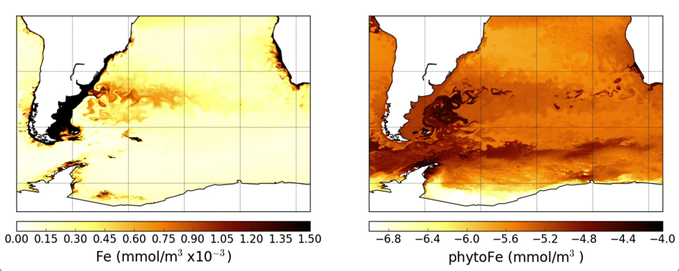
We find that a weak and shallow Atlantic Meridional Overturning Circulation (6-9 Sv, or approximately half of today’s overturning rate) best reproduces the glacial sediment isotope data. Increasing the atmospheric soluble iron flux in the model’s Southern Ocean intensifies export production, carbon storage, and further improves agreement with glacial δ¹³C and δ¹⁵N reconstructions.

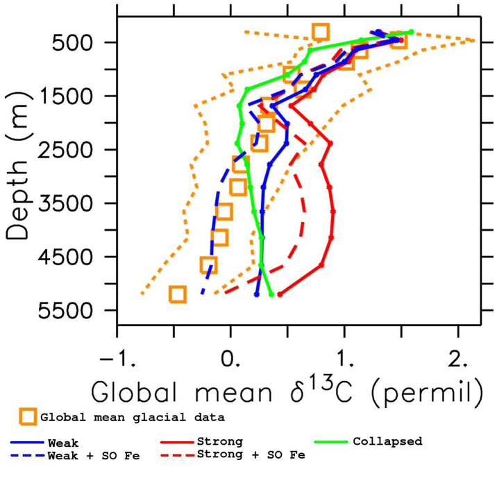
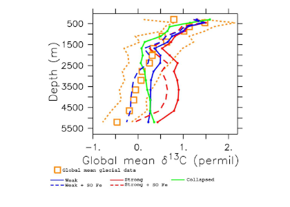
Figure Caption: Depth profiles of global mean δ13C, calculated using only grid boxes for which there exists Last Glacial Maximum data. Blue: Weak Atlantic circulation; Red: Strong Atlantic circulation; Green: Collapsed Atlantic circulation; Dashed: Extra iron in the Southern Ocean; Orange: Last Glacial Maximum Data.

Our best-fitting simulation (blue, dashed line in the figure) is a significant improvement over previous studies and suggests that both circulation and export production changes were necessary to maximize carbon storage in the glacial ocean. These findings provide an equilibrium glacial state, consistent with a combination of proxies, that can be used as a basis for simulations covering the last deglaciation time period. Understanding the different states that the global climate system can transit, and the characteristics of the transitions, is crucial to project possible outcomes of current climate change processes.

Authors:
Juan Muglia (Oregon State University)
Luke C. Skinner (Godwin Laboratory for Palaeoclimate Research, University of Cambridge)
Andreas Schmittner (Oregon State University)

Alternative particle formation pathways identified in the Equatorial Pacific’s biological pump

Posted by mmaheigan

· Tuesday, November 27th, 2018

The ocean is one of the largest sinks of atmospheric carbon dioxide (CO₂) on our planet, driven in part by CO₂uptake by phytoplankton in the upper ocean during photosynthesis. Eventually, a portion of the resulting organic carbon is transported to depth, where it is sequestered from the atmosphere for centuries or even millennia. Our current understanding of the biological pump is based on the export of organic material in the form of large, fast-sinking (hundreds of meters per day) particles. However, using lipids as biomarkers, a recent study from the Equatorial Pacific Ocean published in JGR Biogeosciences showed that fast-sinking particles are refractory and distinctly different from plankton in the mixed layer, whereas slow-sinking particles were more labile and had a more similar composition to mixed layer particles (Fig. 1).

Figure 1. Particle lipid compositions for different particle fractions: ML = homogenous mixed layer particles, SU = suspended, SS = slow-sinking, and FS = fast-sinking of a) labile compounds known as unsaturated fatty acids synthesized by phytoplankton that provide a lot of energy for heterotrophs and b) sterols, including cholesterol (dark blue), which can be a biomarker for heterotrophy. Mixed layer particles are the most labile, showing the least degree of heterotrophic reworking, as expected. However, fast-sinking particles are most dissimilar from those in the mixed layer, with only a small proportion of labile compounds and a high degree of heterotrophic reworking.

The authors proposed a slower, less efficient export pathway, by which phytoplankton initially aggregate to smaller, slower-sinking detrital particles and then gradually form highly degraded, larger particles that sink to depth. Since smaller particles are respired more rapidly than larger particles, the proportion of phytoplankton-captured atmospheric CO₂ being stored in the deep ocean is likely reduced, particularly in regions dominated by smaller phytoplankton such as the Equatorial Pacific. This study clearly demonstrates the need for improved representation of a wider range of particle dynamics in models of the ocean’s biological pump.

Authors:
E. L. Cavan (University of Tasmania, previously University of Southampton)
S. Giering (National Oceanography Centre)
G. Wolff (University of Liverpool)
M. Trimmer (Queen Mary University London)
R. Sanders (National Oceanography Centre)

Improved method to identify and reduce uncertainties in marine carbon cycle predictions

Posted by mmaheigan

· Wednesday, September 26th, 2018

Improved method to identify and reduce uncertainties in marine carbon cycle predictions

How well do contemporary Earth System Models (ESMs) represent the dynamics of the modern day ocean? Often we question the fidelity of biological and chemical processes represented in these ESMs. The fact is representations of biogeochemical processes in models are plagued with some degree of uncertainties; therefore, identifying and reducing such deficiencies could advance ESM development and improve model predictions.

An overview of several models with respect to each of the variables, using absolute (left) and relative (right) scores to determine the degree of uncertainty in relation to referenced datasets.

A recent publication in Atmosphere described the ongoing efforts to develop the International Ocean Model Benchmarking (IOMB) package to evaluate ESM skill sets in simulating marine biogeochemical variables and processes. Model performances were scored based on how well they captured the distribution and variability contained in high-quality observational datasets. The authors highlighted systematic model–data benchmarking as a technique to identify ocean model deficiencies, which could provide a pathway to improving representations of sub-grid-scale parameterizations. They have scaled the absolute score from zero to unity, where the red color tends toward zero to quantify weaknesses in the skill set of a particular model in capturing values from the observational datasets. On the other side of the spectrum, the green color signifies considerable temporal and spatial overlap between the predicted and the observational values. The authors also present the standard score to show the relative scores within two standard deviations from the model mean. The benchmarking package was employed in the published study to assess marine biogeochemical process representations, with a focus on surface ocean concentrations and sea–air fluxes of dimethylsulfide (DMS). The production and emission of natural aerosols remain one of the major limitations in estimating global radiative forcing. Appropriate representation of aerosols in the marine boundary layer (MBL) is essential to reduce uncertainty and provide reliable information on offsets to global warming. Results show that model–data biases increased as DMS enters the MBL, with models over-predicting sea surface concentrations in the productive region of the eastern tropical Pacific by almost a factor of two and the sea–air fluxes by a factor of three. The associated uncertainties with oceanic carbon cycle processes may be additive or antagonistic; in any case, a constructive effort to disentangle the subtleties begins with an objective benchmarking effort, which is focused specifically on marine biogeochemical processes. The tool in development will ensure we satisfy some of the Model Intercomparison Project (MIP) benchmarking needs for the sixth phase of Coupled Model Intercomparison Project (CMIP6).

Authors:
Oluwaseun Ogunro (ORNL)
Scott Elliott (LANL)
Oliver Wingenter (New Mexico Tech)
Clara Deal (University of Alaska)
Weiwei Fu (UC Irvine)
Nathan Collier (ORNL)
Forrest M. Hoffman (ORNL)

When it comes to carbon export, the mesoscale matters

Posted by hbenway

· Tuesday, September 11th, 2018

Figure 1. Difference in annual mean carbon export (ΔPOC flux) between a high resolution (0.1º, Hi-res) and standard resolution (1º, Analog) global climate model simulation using the CESM model. Highlighted regions show areas where vertical (purple boxes) and horizontal (red boxes) changes in nutrient transport drive increases or decreases in export, respectively.

Most Earth System models (ESMs) that are used to study global climate and the carbon cycle do not resolve the most energetic scales in the ocean, the mesoscale (10-100 km), encompassing eddies, coastal jets, and other dynamic features strongly affecting nutrient delivery, productivity, and carbon export. This prompts the question: What are we missing in climate models by not resolving the mesoscale?

Authors of a recent study published in Global Biogeochemical Cycles conducted a comparative analysis of the importance of mesoscale features in biological production and associated carbon export using standard resolution (1°) and mesoscale-resolving (0.1°) ESM simulations. The mesoscale-resolving ESM yielded only a ~2% reduction in globally integrated export production relative to the standard resolution ESM. However, a closer look at the local processes driving export in different basins revealed much larger, compensating differences (Fig. 1). For example, in regions where biological production is driven by natural iron fertilization from shelf sediment sources (Fig. 2), improved representation of coastal jets in the higher-resolution ESM reduces the cross-shelf iron delivery that fuels production (red boxes in Fig. 1). Resolving mesoscale turbulence further reduces the spatial extent of blooms and associated export, yielding a more patchy distribution than in the coarse resolution models. Together, these processes lead to a reduction in export in the Argentine Basin, one of the most productive regions on the planet, of locally up to 50%. In contrast, resolving the mesoscale results in enhanced export production in the Subantarctic (purple box in Fig. 1), where the mesoscale model resolves deeper, narrower mixed layer depths that support stronger nutrient entrainment, in turn enhancing local productivity and export.

Figure 2. An iron-driven plankton bloom structured by mesoscale features in the South Atlantic. Left is simulated dissolved iron (Fe), the limiting nutrient for this region, and right is iron in all phytoplankton classes, a proxy for biomass (phytoFe, shown in log10 scale), on January 11, the height of the bloom. Plankton blooms in the Subantarctic Atlantic are fueled by horizontal iron transport off coastal and island shelves and vertical injection from seamounts, whereas farther south in the Southern Ocean, winter vertical mixing is the primary driver of iron delivery. Mesoscale circulation, largely an unstructured mix of interacting jets and vortices, strongly affects the location and timing of carbon production and export. Click here for an animation.

In regions with very short productivity seasons like the North Pacific and Subantarctic, internally generated mesoscale variability (captured in the higher resolution ESM) yields significant interannual variation in local carbon export. In these regions, a few eddies, filaments or more amorphous mesoscale features can structure the entire production and export pattern for the short bloom season. These findings document the importance of resolving mesoscale features in ESMs to more accurately quantify carbon export, and the different roles mesoscale variability can play in different oceanographic settings.

Determining how to best sample these mesoscale turbulence-dominated blooms and scale up these measurements to regional and longer time means, is an outstanding joint challenge for modelers and observationalists. A key piece is obtaining the high temporal and spatial resolution data sets needed for validating modeled carbon export in bloom regions strongly impacted by mesoscale dynamics, which represent a large portion of the global carbon export.

Authors
Cheryl Harrison (NCAR, University of Colorado Boulder)
Matthew Long (NCAR)
Nicole Lovenduski (University of Colorado Boulder)
J. Keith Moore (University of California Irvine)

Marine Snowfall at the Equator

Posted by mmaheigan

· Thursday, July 19th, 2018

The continual flow of organic particles such as dead organisms and fecal material towards the deep sea is called “marine snow,” and it plays an important role in the ocean carbon cycle and climate-related processes. This snowfall is most intense where high primary production can be observed near the surface. This is the case along the equator in the Pacific and Atlantic Oceans. However, it is not well known how particles are distributed at depth and which processes influence this distribution. A recent study published in Nature Geoscience involved the use of high-resolution particle density data using the Underwater Vision Profiler (UVP) from the equatorial Atlantic and Pacific Oceans down to a depth of 5,000 meters, revealing that several previously accepted ideas on the downward flux of particles into the deep sea should be revisited.

Figure 1. The Underwater Vision Profiler (UVP) during a trial in the Kiel Fjord. The UVP provided crucial data for the new study. Photo: Rainer Kiko, GEOMAR

It is typically assumed that the largest particle density can be found close to the surface and that density attenuates continuously with depth. However, high-resolution particle data show that density increases again in the 300-600-meter depth range. The authors attribute this observation to the daily migratory behavior of organisms such as zooplankton that retreat to these depths during the day, contributing to the particle load via defecation and mortality.

Another surprising result is the observation of many small particles below 1,000 meters depth that contribute a large fraction of the bathypelagic particle flux. This observation counters the general assumption, especially in many biogeochemical models, that particle flux at depth comprises fast sinking particles such as fecal pellets. Diminished remineralization rates of small particles or increased disaggregation of larger particles may contribute to the elevated small particle fluxes at this depth.

Figure 2. Zonal current velocity and Particulate Organic Carbon (POC) content across the equatorial Atlantic at 23˚W as observed in November 2012. From left to right: Zonal current velocity, POC content in small particle fraction and POC content in large particle fraction (adapted from Kiko et al. 2017).

This study highlights the importance of coupled biological and physical processes in understanding and quantifying the biological carbon pump. Further work on this important topic can now also be submitted to the new Frontiers in Marine Science research topic “Zooplankton and Nekton: Gatekeepers of the Biological Pump” (https://www.frontiersin.org/research-topics/8114/zooplankton-and-nekton-gatekeepers-of-the-biological-pump; Co-editors R. Kiko, M. Iversen, A. Maas, H. Hauss and D. Bianchi). The research topic welcomes a broad range of contributions, from individual-based process studies, to local and global field observations, to modeling approaches to better characterize the role of zooplankton and nekton for the biological pump.

Authors:
R. Kiko (GEOMAR)
A. Biastoch (GEOMAR)
P. Brandt (GEOMAR, University of Kiel)
S. Cravatte (LEGOS, University of Toulouse)
H. Hauss (GEOMAR)
R. Hummels (GEOMAR)
I. Kriest (GEOMAR)
F. Marin (LEGOS, University of Toulouse)
A. M. P. McDonnell (University of Alaska Fairbanks)
A. Oschlies (GEOMAR)
M. Picheral (Laboratoire d’Océanographie de Villefranche-sur-Mer, Observatoire Océanologique)
F. U. Schwarzkopf (GEOMAR)
A. M. Thurnherr (Lamont-Doherty Earth Observatory,)
L. Stemmann (Sorbonne Universités, Observatoire Océanologique)

Sensitivity of future ocean acidification to carbon-climate feedbacks

Posted by mmaheigan

· Thursday, May 10th, 2018

There are vast unknowns about the future oceans, from what species or habitats may be most under threat to the continuity of earth system processes that maintain global climate. Modeling can be used to predict future states and explore the impacts of climate change, but several key uncertainties such as carbon-climate feedbacks hamper our predictive power.

Authors of a recent study in Biogeosciences (Matear and Lenton 2018) used a global earth system model to explore the effects of carbon-climate feedbacks on future ocean acidification. Ocean acidification can have wide-ranging impacts on keystone species from reef-building corals to pteropods, a major food web species in the Southern Ocean. The study included four representative scenarios (from IPCC) comparing concentration pathway simulations to emission pathway simulations (RCP2.6, RCP 4.5, RCP6, RCP8.5) to determine carbon-climate feedbacks. The high emission scenarios (RCP8.5 and RCP6) showed surface water undersaturation a decade or more earlier than expected. Surprisingly, the medium (RCP4.5) scenario carbon-climate feedbacks showed the greatest acidification response, doubling the extent of undersaturation and subsequently halving the area that could sustain coral reefs by 2100. The low emissions scenario also showed significant declines in saturation state.

Surface ocean aragonite saturation state for the 2090s for RCP2.6 and RCP 8.5 concentration and emission pathways. The contour line delineates a saturation state of 3 (coral reef threshold), the white line a saturation state of 1, when aragonite becomes unstable and corals dissolve.

The extra atmospheric CO₂ from the carbon-climate feedback resulted in accelerated ocean acidification in all emission scenarios. These feedbacks may also affect global warming and deoxygenation. This is particularly important, given that many policymakers are aiming for low emission commitments, but may still be severely underestimating the extent and timing of ocean acidification. There is a great need to improve our ability to predict carbon-climate feedbacks so we do not underestimate projected ocean acidification and its impacts on both sensitive ecosystems and the human communities that rely on them for food, coastal protection and other ecosystem services.

Authors:
Richard Matear (CSIRO Oceans and Atmosphere, Australia)
Andrew Lenton (Antarctic Climate and Ecosystems CRC, Australia)

Feedbacks mitigate the impacts of atmospheric nitrogen deposition in the western North Atlantic

Posted by mmaheigan

· Thursday, April 12th, 2018

How do phytoplankton respond to atmospheric nitrogen deposition in the western North Atlantic, an area downwind of large agricultural and industrial centers? The biogeochemical impacts of this ‘fertilization’ remain unclear, as direct oceanic observations of atmospheric deposition are limited and models often cannot resolve the important processes.

In a recent study, St-Laurent et al. (2017) simulated the biogeochemical impacts of nitrogen deposition on surface waters of the western North Atlantic by combining year-specific deposition rates from the Community Multiscale Air Quality (CMAQ) model and a realistic 3-D biogeochemical model of the waters off the US east coast. Westerly winds from the continent and large fluxes of heat and moisture over the Gulf Stream produce a ‘hotspot’ of wet nitrogen deposition along the path of the current. This nitrogen input increases the local surface primary productivity by up to 30% during the summer. However, the study also identified important processes that mitigate the impact of atmospheric nitrogen deposition in other seasons and regions. Deposition weakens vertical nitrogen gradients in the upper 20 m and thus decreases the upward transport of nitrogen to the surface layer (a negative feedback). Increases in surface phytoplankton concentrations also negatively impact light availability below the surface through shelf-shading.

Atmospheric nitrogen deposition along the US east coast. (Left) Wet deposition of oxidized nitrogen over the Gulf Stream as simulated by the Community Multiscale Air Quality model (average 2004-2008). (Right) Increase in summer surface primary productivity in response to the deposition (average 2004-2008).

These results indicate that atmospheric nitrogen deposition has important impacts on the surface biogeochemistry of the western North Atlantic but that the response is not simply proportional to the deposition. Additional research is necessary to clarify the role played by atmospheric deposition in this region in past and future centuries. While inputs of atmospheric nitrogen associated with power plants and industries have decreased since the passage of the Clean Air Act, recent studies have revealed increasing atmospheric concentrations of reduced nitrogen. Continued coordination between modeling and observing efforts (both on land and over the ocean) are needed to improve our understanding of the impacts of deposition on the biological pump in this region of the Atlantic ocean.

Authors:
Pierre St-Laurent (VIMS, College of William and Mary)
Marjorie A.M. Friedrichs (VIMS, College of William and Mary)
Raymond G. Najjar (Pennsylvania State University)
Doug Martins (FLIR Systems Inc.)
Maria Herrmann (Pennsylvania State University)
Sonya K. Miller (Pennsylvania State University)
John Wilkin (Rutgers University)

Volcanic carbon dioxide drove ancient global warming event

Posted by mmaheigan

· Thursday, March 29th, 2018

A study recently published in Nature suggests that an extreme global warming event 56 million years ago known as the Palaeocene-Eocene Thermal Maximum (PETM) was driven by massive CO₂ emissions from volcanoes during the formation of the North Atlantic Ocean. Using a combination of new geochemical measurements and novel global climate modelling, the study revealed that atmospheric CO₂ more than doubled in less than 25,000 years during the PETM.

The PETM lasted ~150,000 years and is the most rapid and extreme natural global warming event of the last 66 million years. During the PETM, global temperatures increased by at least 5^°C, comparable to temperatures projected in the next century and beyond. While it has long been suggested that the PETM event was caused by the injection of carbon into the ocean and atmosphere, the source and total amount of carbon, as well as the underlying mechanism have thus far remained elusive. The PETM roughly coincided with the formation of massive flood basalts resulting from of a series of eruptions that occurred as Greenland and North America started separating from Europe, thereby creating the North Atlantic Ocean. What was missing is evidence linking the volcanic activity to the carbon release and warming that marks the PETM.

To identify the source of carbon, the authors measured changes in the balance of isotopes of the element boron in ancient sediment-bound marine fossils called foraminifera to generate a new record of ocean pH throughout the PETM. Ocean pH tells us about the amount of carbon absorbed by ancient seawater, but we can get even more information by also considering changes in the isotopes of carbon, which provide information about the carbon source. When forced with these ocean pH and carbon isotope data, a numerical global climate model implicates large-scale volcanism associated with the opening of the North Atlantic as the primary driver of the PETM.

North Atlantic microfossil-derived isotope records from extinct planktonic foraminiferal species M. subbotinae relative to the onset of the PETM carbon isotope excursion (CIE). The negative trend in carbon isotope composition (A) during the carbon emission phase is accompanied by decreasing pH (decreasing δ¹¹B, panel B) and increasing temperature (decreasing δ¹⁸O, panel C). Panels D and E zoom in on the PETM CIE, showing microfossil δ¹³C (D) and δ¹¹B-based pH (E) reconstructions. Also included in E are data from Penman et al. (2014) on their original age model, with recalculated (lab-based) pH values.

These new results suggest that the PETM was associated with a total input of >12,000 petagrams of carbon from a predominantly volcanic source. This is a vast amount of carbon—30 times larger than all of the fossil fuels burned to date and equivalent to all current conventional and unconventional fossil fuel reserves. In the following Earth System Model simulations, it resulted in the concentration of atmospheric CO₂ increasing from ~850 parts per million to >2000 ppm. The Earth’s mantle contains more than enough carbon to explain this dramatic rise, and it would have been released as magma poured from volcanic rifts at the Earth’s surface.

How the ancient Earth system responded to this carbon injection at the PETM can tell us a great deal about how it might respond in the future to man-made climate change. Earth’s warming at the PETM was about what we would expect given the CO₂ emitted and what we know about the sensitivity of the climate system based on Intergovernmental Panel on Climate Change (IPCC) reports. However, the rate of carbon addition during the PETM was about twenty times slower than today’s human-made carbon emissions.

In the model outputs, carbon cycle feedbacks such as methane release from gas hydrates—once the favoured explanation of the PETM—did not play a major role in driving the event. Additionally, one unexpected result was that enhanced organic matter burial was important in ultimately drawing down the released carbon out of the atmosphere and ocean and thereby accelerating the recovery of the Earth system.

Authors:
Marcus Gutjahr (National Oceanography Centre Southamption, GEOMAR)
Andy Ridgwell (Bristol University, University of California Riverside)
Philip F. Sexton (The Open University, UK)
Eleni Anagnostou (National Oceanography Centre Southamption)
Paul N. Pearson (Cardiff University)
Heiko Pälike (University of Bremen)
Richard D. Norris (Scripps Institution of Oceanography)
Ellen Thomas (Yale University, Wesleyan University)
Gavin L. Foster (National Oceanography Centre Southamption)

Widespread nutrient co-limitation discovered in the South Atlantic

Posted by mmaheigan

· Thursday, March 15th, 2018

Unicellular photosynthetic microbes—phytoplankton—are responsible for virtually all oceanic primary production, which fuels marine food webs and plays a fundamental role in the global carbon cycle. Experiments to date have suggested that the growth of phytoplankton across much of the ocean is limited by either nitrogen or iron. But simultaneously low concentrations of these and other nutrients have been measured over large areas of the open ocean, raising the question: Are phytoplankton communities only limited by a single nutrient?

Authors of a study recently published in Nature tested this by conducting nutrient addition experiments on a GEOTRACES cruise in the nutrient-deficient South Atlantic gyre. Seawater samples were amended with nitrogen, iron, and cobalt both individually and in various combinations. Concurrent nitrogen and iron addition stimulated increased phytoplankton growth, yielding a ~40-fold increase in chlorophyll a. Supplementary addition of cobalt or cobalt-containing vitamin B₁₂ further enhanced phytoplankton growth in several experiments.

Experiments conducted throughout the southeast Atlantic GEOTRACES GA08 cruise transect (left panel) demonstrated that nitrogen and iron had to be added to significantly stimulate phytoplankton growth (right panel). Supplementary addition of cobalt (or cobalt-containing vitamin B12) stimulated significant additional growth.

In addition to co-limited sites, the study identified ‘singly’ and ‘serially’ limited sites. These limitation regimes could be predicted by the measured ambient seawater nutrient concentrations, demonstrating the potential for using nutrient datasets to make confident predictions about limitation at larger spatial scales, an approach that is being more widely used in programmes like GEOTRACES,.

Finally, a complex, state-of-the-art biogeochemical ocean model suggested a much smaller extent of nutrient co-limitation than the experiments indicated. Authors attributed this to relatively restricted microbial and nutrient diversity in the model. These findings have implications for how such models are constructed if they are to represent nutrient co-limitation in the ocean and accurately project changes in ocean productivity in the future.

Authors:
Thomas J. Browning (GEOMAR)
Eric P. Achterberg (GEOMAR)
Insa Rapp (GEOMAR)
Anja Engel (GEOMAR)
Erin M. Bertrand (Dalhousie University)
Alessandro Tagliabue (University of Liverpool)
Mark Moore (University of Southampton)

Increased temperatures suggest reduced capacity for carbon

Posted by mmaheigan

· Thursday, January 18th, 2018

The ocean’s biological pump works to draw down atmospheric carbon dioxide (CO₂) by exporting carbon from the surface ocean. This process is less efficient at higher temperatures, implying a possible climate feedback. Recent work by Cael et al. provides an explanation of why this feedback occurs and an estimate of its severity.

In a highly simplified view, carbon export depends on the balance between two temperature-dependent processes: 1) The autotrophic production and 2) the heterotrophic respiration of organic carbon. Cael and Follows (Geophysical Research Letters 2016) recently developed a mechanistic model based on established temperature dependencies for photosynthesis and respiration to explore feedbacks between export efficiency and climate. Heterotrophic growth rates increase more so than phototrophic rates with increasing temperature, which suggests that at higher temperatures, community respiration will increase relative to production, thereby decreasing export efficiency. Although simplistic, the model captures the temperature dependence of export efficiency observations.

Figure: Schematic of the mechanism on which the Cael and Follows (2016) model is based. (a) Photosynthesis (dark grey) and respiration (light grey) respond to temperature differently, yielding (b) a decline in export efficiency at higher temperatures.

More recently, Cael, Bisson, and Follows (Limnology and Oceanography 2017) applied this model to sea surface temperature records and estimated a ~1.5% decline in globally-averaged export efficiency over the past three decades of increasing ocean temperatures as a result of this metabolic mechanism. This ~1.5% decline is equivalent to a reduced ocean sequestration of approximately 100 million fewer tons of carbon annually, comparable to the annual carbon emissions of the United Kingdom. The model provides a framework in which to consider the relationship between climate and ocean carbon export that might also elucidate large-scale (e.g., glacial-interglacial) atmospheric CO₂ changes of the past.

Authors:
B. B. Cael (MIT/WHOI)
Kelsey Bisson (UCSB)
Mick Follows (MIT)

Funding for the Ocean Carbon & Biogeochemistry Project Office is provided by the National Science Foundation (NSF) and the National Aeronautics and Space Administration (NASA). The OCB Project Office is housed at the Woods Hole Oceanographic Institution.

Archive for modeling – Page 6

Filter by Keyword