modeling :: Ocean Carbon & Biogeochemistry

Studying marine ecosystems and biogeochemical cycles in the face of environmental change

Archive for modeling – Page 7

Feedbacks mitigate the impacts of atmospheric nitrogen deposition in the western North Atlantic

Posted by mmaheigan

· Thursday, April 12th, 2018

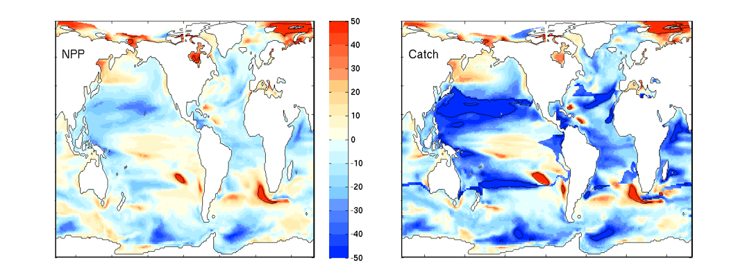
How do phytoplankton respond to atmospheric nitrogen deposition in the western North Atlantic, an area downwind of large agricultural and industrial centers? The biogeochemical impacts of this ‘fertilization’ remain unclear, as direct oceanic observations of atmospheric deposition are limited and models often cannot resolve the important processes.

In a recent study, St-Laurent et al. (2017) simulated the biogeochemical impacts of nitrogen deposition on surface waters of the western North Atlantic by combining year-specific deposition rates from the Community Multiscale Air Quality (CMAQ) model and a realistic 3-D biogeochemical model of the waters off the US east coast. Westerly winds from the continent and large fluxes of heat and moisture over the Gulf Stream produce a ‘hotspot’ of wet nitrogen deposition along the path of the current. This nitrogen input increases the local surface primary productivity by up to 30% during the summer. However, the study also identified important processes that mitigate the impact of atmospheric nitrogen deposition in other seasons and regions. Deposition weakens vertical nitrogen gradients in the upper 20 m and thus decreases the upward transport of nitrogen to the surface layer (a negative feedback). Increases in surface phytoplankton concentrations also negatively impact light availability below the surface through shelf-shading.

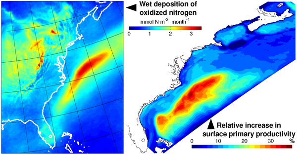
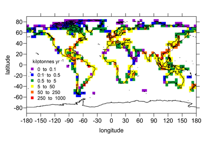
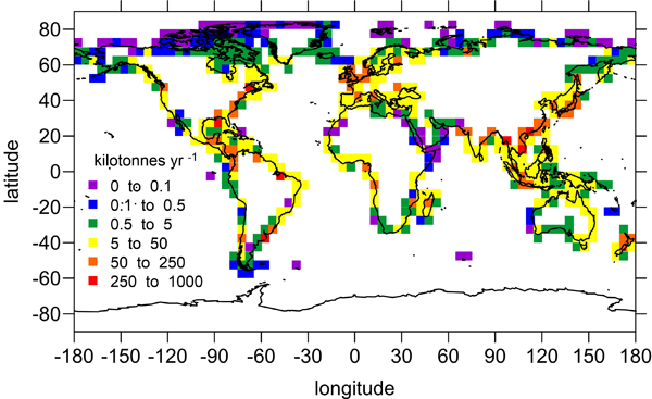
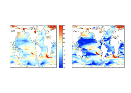
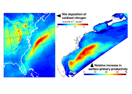
Atmospheric nitrogen deposition along the US east coast. (Left) Wet deposition of oxidized nitrogen over the Gulf Stream as simulated by the Community Multiscale Air Quality model (average 2004-2008). (Right) Increase in summer surface primary productivity in response to the deposition (average 2004-2008).

These results indicate that atmospheric nitrogen deposition has important impacts on the surface biogeochemistry of the western North Atlantic but that the response is not simply proportional to the deposition. Additional research is necessary to clarify the role played by atmospheric deposition in this region in past and future centuries. While inputs of atmospheric nitrogen associated with power plants and industries have decreased since the passage of the Clean Air Act, recent studies have revealed increasing atmospheric concentrations of reduced nitrogen. Continued coordination between modeling and observing efforts (both on land and over the ocean) are needed to improve our understanding of the impacts of deposition on the biological pump in this region of the Atlantic ocean.

Authors:
Pierre St-Laurent (VIMS, College of William and Mary)
Marjorie A.M. Friedrichs (VIMS, College of William and Mary)
Raymond G. Najjar (Pennsylvania State University)
Doug Martins (FLIR Systems Inc.)
Maria Herrmann (Pennsylvania State University)
Sonya K. Miller (Pennsylvania State University)
John Wilkin (Rutgers University)

Volcanic carbon dioxide drove ancient global warming event

Posted by mmaheigan

· Thursday, March 29th, 2018

A study recently published in Nature suggests that an extreme global warming event 56 million years ago known as the Palaeocene-Eocene Thermal Maximum (PETM) was driven by massive CO₂ emissions from volcanoes during the formation of the North Atlantic Ocean. Using a combination of new geochemical measurements and novel global climate modelling, the study revealed that atmospheric CO₂ more than doubled in less than 25,000 years during the PETM.

The PETM lasted ~150,000 years and is the most rapid and extreme natural global warming event of the last 66 million years. During the PETM, global temperatures increased by at least 5^°C, comparable to temperatures projected in the next century and beyond. While it has long been suggested that the PETM event was caused by the injection of carbon into the ocean and atmosphere, the source and total amount of carbon, as well as the underlying mechanism have thus far remained elusive. The PETM roughly coincided with the formation of massive flood basalts resulting from of a series of eruptions that occurred as Greenland and North America started separating from Europe, thereby creating the North Atlantic Ocean. What was missing is evidence linking the volcanic activity to the carbon release and warming that marks the PETM.

To identify the source of carbon, the authors measured changes in the balance of isotopes of the element boron in ancient sediment-bound marine fossils called foraminifera to generate a new record of ocean pH throughout the PETM. Ocean pH tells us about the amount of carbon absorbed by ancient seawater, but we can get even more information by also considering changes in the isotopes of carbon, which provide information about the carbon source. When forced with these ocean pH and carbon isotope data, a numerical global climate model implicates large-scale volcanism associated with the opening of the North Atlantic as the primary driver of the PETM.

North Atlantic microfossil-derived isotope records from extinct planktonic foraminiferal species M. subbotinae relative to the onset of the PETM carbon isotope excursion (CIE). The negative trend in carbon isotope composition (A) during the carbon emission phase is accompanied by decreasing pH (decreasing δ¹¹B, panel B) and increasing temperature (decreasing δ¹⁸O, panel C). Panels D and E zoom in on the PETM CIE, showing microfossil δ¹³C (D) and δ¹¹B-based pH (E) reconstructions. Also included in E are data from Penman et al. (2014) on their original age model, with recalculated (lab-based) pH values.

These new results suggest that the PETM was associated with a total input of >12,000 petagrams of carbon from a predominantly volcanic source. This is a vast amount of carbon—30 times larger than all of the fossil fuels burned to date and equivalent to all current conventional and unconventional fossil fuel reserves. In the following Earth System Model simulations, it resulted in the concentration of atmospheric CO₂ increasing from ~850 parts per million to >2000 ppm. The Earth’s mantle contains more than enough carbon to explain this dramatic rise, and it would have been released as magma poured from volcanic rifts at the Earth’s surface.

How the ancient Earth system responded to this carbon injection at the PETM can tell us a great deal about how it might respond in the future to man-made climate change. Earth’s warming at the PETM was about what we would expect given the CO₂ emitted and what we know about the sensitivity of the climate system based on Intergovernmental Panel on Climate Change (IPCC) reports. However, the rate of carbon addition during the PETM was about twenty times slower than today’s human-made carbon emissions.

In the model outputs, carbon cycle feedbacks such as methane release from gas hydrates—once the favoured explanation of the PETM—did not play a major role in driving the event. Additionally, one unexpected result was that enhanced organic matter burial was important in ultimately drawing down the released carbon out of the atmosphere and ocean and thereby accelerating the recovery of the Earth system.

Authors:
Marcus Gutjahr (National Oceanography Centre Southamption, GEOMAR)
Andy Ridgwell (Bristol University, University of California Riverside)
Philip F. Sexton (The Open University, UK)
Eleni Anagnostou (National Oceanography Centre Southamption)
Paul N. Pearson (Cardiff University)
Heiko Pälike (University of Bremen)
Richard D. Norris (Scripps Institution of Oceanography)
Ellen Thomas (Yale University, Wesleyan University)
Gavin L. Foster (National Oceanography Centre Southamption)

Widespread nutrient co-limitation discovered in the South Atlantic

Posted by mmaheigan

· Thursday, March 15th, 2018

Unicellular photosynthetic microbes—phytoplankton—are responsible for virtually all oceanic primary production, which fuels marine food webs and plays a fundamental role in the global carbon cycle. Experiments to date have suggested that the growth of phytoplankton across much of the ocean is limited by either nitrogen or iron. But simultaneously low concentrations of these and other nutrients have been measured over large areas of the open ocean, raising the question: Are phytoplankton communities only limited by a single nutrient?

Authors of a study recently published in Nature tested this by conducting nutrient addition experiments on a GEOTRACES cruise in the nutrient-deficient South Atlantic gyre. Seawater samples were amended with nitrogen, iron, and cobalt both individually and in various combinations. Concurrent nitrogen and iron addition stimulated increased phytoplankton growth, yielding a ~40-fold increase in chlorophyll a. Supplementary addition of cobalt or cobalt-containing vitamin B₁₂ further enhanced phytoplankton growth in several experiments.

Experiments conducted throughout the southeast Atlantic GEOTRACES GA08 cruise transect (left panel) demonstrated that nitrogen and iron had to be added to significantly stimulate phytoplankton growth (right panel). Supplementary addition of cobalt (or cobalt-containing vitamin B12) stimulated significant additional growth.

In addition to co-limited sites, the study identified ‘singly’ and ‘serially’ limited sites. These limitation regimes could be predicted by the measured ambient seawater nutrient concentrations, demonstrating the potential for using nutrient datasets to make confident predictions about limitation at larger spatial scales, an approach that is being more widely used in programmes like GEOTRACES,.

Finally, a complex, state-of-the-art biogeochemical ocean model suggested a much smaller extent of nutrient co-limitation than the experiments indicated. Authors attributed this to relatively restricted microbial and nutrient diversity in the model. These findings have implications for how such models are constructed if they are to represent nutrient co-limitation in the ocean and accurately project changes in ocean productivity in the future.

Authors:
Thomas J. Browning (GEOMAR)
Eric P. Achterberg (GEOMAR)
Insa Rapp (GEOMAR)
Anja Engel (GEOMAR)
Erin M. Bertrand (Dalhousie University)
Alessandro Tagliabue (University of Liverpool)
Mark Moore (University of Southampton)

Increased temperatures suggest reduced capacity for carbon

Posted by mmaheigan

· Thursday, January 18th, 2018

The ocean’s biological pump works to draw down atmospheric carbon dioxide (CO₂) by exporting carbon from the surface ocean. This process is less efficient at higher temperatures, implying a possible climate feedback. Recent work by Cael et al. provides an explanation of why this feedback occurs and an estimate of its severity.

In a highly simplified view, carbon export depends on the balance between two temperature-dependent processes: 1) The autotrophic production and 2) the heterotrophic respiration of organic carbon. Cael and Follows (Geophysical Research Letters 2016) recently developed a mechanistic model based on established temperature dependencies for photosynthesis and respiration to explore feedbacks between export efficiency and climate. Heterotrophic growth rates increase more so than phototrophic rates with increasing temperature, which suggests that at higher temperatures, community respiration will increase relative to production, thereby decreasing export efficiency. Although simplistic, the model captures the temperature dependence of export efficiency observations.

Figure: Schematic of the mechanism on which the Cael and Follows (2016) model is based. (a) Photosynthesis (dark grey) and respiration (light grey) respond to temperature differently, yielding (b) a decline in export efficiency at higher temperatures.

More recently, Cael, Bisson, and Follows (Limnology and Oceanography 2017) applied this model to sea surface temperature records and estimated a ~1.5% decline in globally-averaged export efficiency over the past three decades of increasing ocean temperatures as a result of this metabolic mechanism. This ~1.5% decline is equivalent to a reduced ocean sequestration of approximately 100 million fewer tons of carbon annually, comparable to the annual carbon emissions of the United Kingdom. The model provides a framework in which to consider the relationship between climate and ocean carbon export that might also elucidate large-scale (e.g., glacial-interglacial) atmospheric CO₂ changes of the past.

Authors:
B. B. Cael (MIT/WHOI)
Kelsey Bisson (UCSB)
Mick Follows (MIT)

WBC Series: Decadal variability of the Kuroshio Extension system and its impact on subtropical mode water formation

Posted by mmaheigan

· Friday, November 10th, 2017

Bo Qiu¹, Eitarou Oka², Stuart P. Bishop³, Shuiming Chen¹, Andrea J. Fassbender⁴

1. University of Hawaii at Manoa
2. The University of Tokyo
3. North Carolina State University
4. Monterey Bay Aquarium Research Institute

After separating from the Japanese coast at 36°N, 141°E, the Kuroshio enters the open basin of the North Pacific, where it is renamed the Kuroshio Extension (KE). Free from the constraint of coastal boundaries, the KE has been observed to be an eastward-flowing inertial jet accompanied by large-amplitude meanders and energetic pinched-off eddies (see Qiu 2002 and Kelly et al. 2010 for comprehensive reviews). Compared to its upstream counterpart south of Japan, the Kuroshio, the KE is accompanied by a stronger southern recirculation gyre that increases the KE’s eastward volume transport to more than twice the maximum Sverdrup transport (~ 60Sv) in the subtropical North Pacific Ocean (Wijffels et al. 1998). This has two important consequences. Dynamically, the increased transport enhances the nonlinearity of the KE jet, rendering the region surrounding the KE jet to have the highest mesoscale activity level in the Pacific basin. Thermodynamically, the enhanced KE jet brings a significant amount of tropical-origin warm water to the mid-latitude ocean to be in direct contact with cold, dry air blowing off the Eurasian continent. This results in significant wintertime heat loss from the ocean to atmosphere surrounding the Kuroshio/KE paths, contributing to the formation of North Pacific subtropical mode water (STMW; see Hanawa and Talley (2001) and Oka and Qiu (2012) for comprehensive reviews).

Figure 1. Yearly paths of the Kuroshio and KE plotted every 14 days using satellite SSH data (updated based on Qiu and Chen 2005). KE was in stable state in 1993–94, 2002–05, and 2010–15, and unstable state in 1995-2001, 2006–09, and 2016, respectively.

Although the ocean is known to be a turbulent medium, variations in both the level of mesoscale eddy activity and the formation rate of STMW in the KE region are by no means random on interannual and longer timescales. One important feature emerging from recent satellite altimeter measurements and eddy-resolving ocean model simulations is that the KE system exhibits clearly defined decadal modulations between a stable and an unstable dynamical state (e.g., Qiu & Chen 2005, 2010; Taguchi et al. 2007; Qiu et al. 2007; Cebollas et al. 2009; Sugimoto and Hanawa 2009; Sasaki et al. 2013; Pierini 2014; Bishop et al. 2015). As shown in Figure 1, the KE paths were relatively stable in 1993–95, 2002–05, and 2010–15. In contrast, spatially convoluted paths prevailed during 1996–2001 and 2006–09. When the KE jet is in a stable dynamical state, satellite altimeter data further reveal that its eastward transport and latitudinal position tend to increase and migrate northward, its southern recirculation gyre tends to strengthen, and the regional eddy kinetic energy level tends to decrease. The reverse is true when the KE jet switches to an unstable dynamical state. In fact, the time-varying dynamical state of the KE system can be well represented by the KE index, defined by the average of the variance-normalized time series of the southern recirculation gyre intensity, the KE jet intensity, its latitudinal position, and the negative of its path length (Qiu et al. 2014). Figure 2a shows the KE index time series in the satellite altimetry period of 1993–present; here, a positive KE index indicates a stable dynamical state and a negative KE index, an unstable dynamical state. From Figure 2a, it is easy to discern the dominance of the decadal oscillations between the two dynamical states of the KE system.

Figure 2. (a) Time series of the KE index from 1993‑present; available at http://www.soest.hawaii.edu/oceanography/bo/KE_index.asc. (b) Year-mean SSH maps when the KE is in stable (2004 and 2011) versus unstable (1997 and 2008) states. (c) SSH anomalies along the zonal band of 32°-34°N from satellite altimetry measurements. (d) Time series of the PDO index from 1989-present; available at http://jisao.washington.edu/pdo/PDO.latest.

Transitions between the KE’s two dynamical states are caused by the basin-scale wind stress curl forcing in the eastern North Pacific related to the Pacific Decadal Oscillation (PDO). Specifically, when the central North Pacific wind stress curl anomalies are positive during the positive PDO phase (see Figure 2d), enhanced Ekman flux divergence generates negative local sea surface height (SSH) anomalies in 170°–150°W along the southern recirculation gyre latitude of 32°–34°N. As these wind-induced negative SSH anomalies propagate westward as baroclinic Rossby waves into the KE region after a delay of 3–4 years (Figure 2c), they weaken the zonal KE jet, leading to an unstable (i.e., negative index) state of the KE system with a reduced recirculation gyre and an active eddy kinetic energy field (Figure 2b). Negative anomalous wind stress curl forcing during the negative PDO phase, on the other hand, generates positive SSH anomalies through the Ekman flux convergence in the eastern North Pacific. After propagating into the KE region in the west, these anomalies stabilize the KE system by increasing the KE transport and by shifting its position northward, leading to a positive index state.

The dynamical state of the KE system exerts a tremendous influence upon the STMW that forms largely along the paths of the Kuroshio/KE jet and inside of its southern recirculation gyre (e.g., Suga et al. 2004; Qiu et al. 2006; Oka 2009). Figure 3a shows the monthly time series of temperature profile, constructed by averaging available Argo and XBT/CTD/XCTD data inside the KE southern recirculation gyre (see Qiu and Chen 2006 for details on the constructing method). The black line in the plot denotes the base of the mixed layer, defined as where the water temperature drops by 0.5°C from the sea surface temperature. Based on the temperature profiles, Figure 3b shows the monthly time series of potential vorticity. STMW in Figure 3b is characterized by water columns with potential vorticity of less than 2.0 x 10^-10 m^-1s^-1 beneath the mixed layer. From Figure 3, it is clear that both the late winter mixed layer depth and the low-potential vorticity STMW layer underwent significant decadal changes over the past 25 years. Specifically, deep mixed layer and pronounced low-potential vorticity STMW were detected in 1993–95, 2001–05, and 2010–15, and these years corresponded roughly to the periods when the KE index was in the positive phase (cf. Figure 2a).

Figure 3. Monthly time series of (a) temperature (°C) and (b) potential vorticity (10-10 m-1 s-1) averaged in the KE’s southern recirculation gyre. The thick black and white lines in (a) and (b) denote the base of the mixed layer, defined as where the temperature drops by 0.5°C from the surface value. Red pluses (at the top of each panel) indicate the individual temperature profiles used in constructing the monthly T(z, t) profiles. The potential vorticity, Q(z,t) = fα∂T(z,t)/∂z, where f is the Coriolis parameter and α the thermal expansion coefficient.

The close connection between the dynamical state of the KE system and the STMW formation has been detected by many recent studies based on different observational data sources and analysis approaches (Qiu and Chen 2006; Sugimoto and Hanawa 2010; Rainville et al. 2014; Bishop and Watts 2014; Oka et al. 2012; 2015; Cerovecki and Giglio 2016). Physically, this connection can be understood as follows. When the KE is in an unstable state (or a negative KE index phase), high-regional eddy variability infuses high-potential vorticity KE and subarctic-gyre water into the southern recirculation gyre, increasing the upper-ocean stratification and hindering the development of deep winter mixed layer and formation of STMW. A stable KE path with suppressed eddy variability (in the positive KE index phase), on the other hand, favors the maintenance of a weak stratification in the recirculation gyre, leading to the formation of a deep winter mixed layer and thick STMW.

Since the STMW is renewed each winter, due to combined net surface heat flux and wind stress forcing that modulate on interannual timescales, a question arising naturally is the timescale on which the dynamical state change of the KE system is able to alter the upper ocean stratification and potential vorticity inside the recirculation gyre. If the influence of the KE dynamical state acts on interannual timescales, one may expect a stronger control on the STMW variability by the wintertime atmospheric condition (e.g., Suga and Hanawa 1995; Davis et al. 2011). Intensive observations from the Kuroshio Extension System Study (KESS) program, spanning the period from April 2004 to July 2006, captured the 2004–05 transition of the KE system from a stable to an unstable state. The combined measurements by profiling Argo floats, moored current meter, current and pressure inverted echo sounder (CPIES), and the Kuroshio Extension Observatory (KEO) surface mooring revealed that the KE dynamical state change was able to change the STMW properties both significantly in amplitude and effectively in time (Qiu et al. 2007; Bishop 2013; Cronin et al. 2013; Bishop and Watts 2014). Relative to 2004, the low-potential vorticity signal in the core of STMW was diminished by one-half in 2005, and this weakening of STMW’s intensity occurred within a period of less than seven months. These significant and rapid responses of STMW to the KE dynamical state change suggests that the variability in STMW formation is more sensitive to the dynamical state of the KE than to interannual variations in overlying atmospheric conditions over the past 25 years.

The decadal variability of STMW in the KE’s southern recirculation gyre is able to affect the water property distributions in the entire western part of the North Pacific subtropical gyre (Oka et al. 2015). Measurements by Argo profiling floats during 2005–14 revealed that the volume and spatial extent of STMW decreased (increased) in 2006–09 (after 2010) during the unstable (stable) KE period in its formation region north of ~28°N, as well as in the southern, downstream regions with a time lag of 1-2 years. Such decadal subduction variability affects not only physical but also biogeochemical structures in the downstream, interior subtropical gyre. Shipboard observations at 25°N and along the 137°E repeat hydrographic section of the Japan Meteorological Agency exhibited that, after 2010, enhanced subduction of STMW consistently increased dissolved oxygen, pH, and aragonite saturation state and decreased potential vorticity, apparent oxygen utilization, nitrate, and dissolved inorganic carbon. Changes in dissolved inorganic carbon, pH, and aragonite saturation state were opposite their long-term trends.

KE State and the Ocean Carbon Cycle

Western boundary current (WBC) regions display the largest magnitude air-to-sea carbon dioxide (CO₂) fluxes of anywhere in the global ocean. STMW formation processes are thought to account for a majority of the anthropogenic CO₂ sequestration that occurs outside of the polar, deep water formation regions (Sabine et al. 2004; Khatiwala et al. 2009). Once subducted and advected away from the formation region, mode waters often remain out of contact with the atmosphere on timescales of decades to hundreds of years, making them short-term carbon silos relative to the abyssal carbon storage reservoirs. One of the physical impacts on carbon uptake via air-sea CO₂flux is due to the temperature dependence of the solubility of pCO₂ in the surface waters. Cooler surface waters during the wintertime months reduce the oceanic pCO₂and subsequently enhance the CO₂flux into the ocean. This carbon uptake corresponds with the timing of peak STMW formation.

As mentioned above, the formation of STMW is modulated by the dynamic states of the KE, with less STMW forming during unstable states and more during stable states. To complicate matters, more enhanced levels of surface chlorophyll (Chla) have also been observed from satellite ocean color during unstable states (Lin et al. 2014), which points to the potential importance of biophysical interactions on carbon uptake. Elevated levels of Chla can further modify the pCO₂ of surface waters and enhance carbon export at depth from sinking of particulate organic matter following an individual bloom. Given that submesoscale processes result from deep wintertime mixed layers and from the presence of the larger mesoscale lateral shear and strain fields (McWilliams 2016), it is expected that submesoscale processes are also important in STMW formation during unstable states of the KE. An open question in the research community is to what extent do elevated levels of mesoscale and submesoscale eddy activity modulate STMW formation and carbon uptake during unstable states of the KE? With large variations in STMW formation occurring in concert with decadal variability in the mesoscale eddy field, it is possible that submesoscale processes may impact STMW formation through restratification of the mixed layer within density classes encompassing STMW and timing of the spring bloom. These mesoscale and submesoscale processes may then also impact the uptake of CO₂ in the North Pacific on interannual to decadal timescales.

References

Bishop, S. P., 2013: Divergent eddy heat fluxes in the Kuroshio Extension at 143°-149°E. Part II: Spatiotemporal variability. J. Phys. Oceanogr., 43, 2416-2431, doi: 10.1175/JPO-D-13-061.1.

Bishop, S. P., and D. R. Watts, 2014: Rapid eddy-induced modification of subtropical mode water during the Kuroshio Extension System Study. J. Phys. Oceanogr., 44, 1941-1953, doi:10.1175/JPO-D-13-0191.1.

Bishop, S. P., F. O. Bryan, and R. J. Small, 2015: Bjerknes-like compensation in the wintertime north Pacific. J. Phys. Oceanogr., 45, 1339-1355, doi:10.1175/JPO-D-14-0157.1.

Ceballos, L., E. Di Lorenzo, C. D. Hoyos, N. Schneider, and B. Taguchi, 2009: North Pacific Gyre oscillation synchronizes climate variability in the eastern and western boundary current systems. J. Climate, 22, 5163-5174, doi:10.1175/2009JCLI2848.1.

Cerovecki, I., and D. Giglio, 2016: North Pacific subtropical mode water volume decrease in 2006–09 estimated from Argo observations: Influence of surface formation and basin-scale oceanic variability. J. Climate, 29, 2177-2199, doi:10.1175/JCLI-D-15-0179.1.

Cronin, M. F., N. A. Bond, J. T. Farrar, H. Ichikawa, S. R. Jayne, Y. Kawai, M. Konda, B. Qiu, L. Rainville, and H. Tomita, 2013: Formation and erosion of the seasonal thermocline in the Kuroshio Extension Recirculation Gyre. Deep-Sea Res. II, 85, 62-74, doi:10.1016/j.dsr2.2012.07.018.

Davis, X. J., L. M. Rothstein, W. K. Dewar, and D. Menemenlis, 2011: Numerical investigations of seasonal and interannual variability of North Pacific subtropical mode water and its implications for Pacific climate variability. J. Climate, 24, 2648-2665, doi:10.1175/2010JCLI3435.1.

Hanawa, K., and L. D. Talley, 2001: Mode waters. Ocean Circulation and Climate: Observing and Modelling the Global Ocean, G. Siedler, J. Church, and J. Gould, Eds., Academic Press, 373-386.

Khatiwala, S., Primeau, F., and Hall, T., 2009: Reconstruction of the history of anthropogenic CO2 concentrations in the ocean. Nature, 462, 346–349, doi:10.1038/nature08526.

Kelly, K. A., R. J. Small, R. M. Samelson, B. Qiu, T. M. Joyce, Y.-O. Kwon, and M. F. Cronin, 2010: Western boundary currents and frontal air-sea interaction: Gulf Stream and Kuroshio Extension. J. Climate, 23, 5644-5667, doi:10.1175/2010JCLI3346.1.

Lin, P., F. Chai, H. Xue, and P. Xiu, 2014: Modulation of decadal oscillation on surface chlorophyll in the Kuroshio Extension. J. Geophys. Res., 119, 187–199, doi:10.1002/2013JC009359.

McWilliams, J. C., 2016: Submesoscale currents in the ocean. Proc. Roy. Soc. A, 472, doi:10.1098/rspa.2016.0117..

Oka, E., 2009: Seasonal and interannual variation of North Pacific subtropical mode water in 2003–2006. J. Oceanogr., 65, 151-164, doi:10.1007/s10872-009-0015-y.

Oka, E., and B. Qiu, 2012: Progress of North Pacific mode water research in the past decade. J. Oceanogr., 68, 5-20, doi:10.1007/s10872-011-0032-5.

Oka, E., B. Qiu, S. Kouketsu, K. Uehara, and T. Suga, 2012: Decadal seesaw of the central and subtropical mode water formation associated with the Kuroshio Extension variability. J. Oceanogr., 68, 355-360, doi: 10.1007/s10872-015-0300-x.

Oka, E., B. Qiu, Y. Takatani, K. Enyo, D. Sasano, N. Kosugi, M. Ishii, T. Nakano, and T. Suga, 2015: Decadal variability of subtropical mode water subduction and its impact on biogeochemistry. J. Oceanogr., 71, 389-400, doi: 10.1007/s10872-015-0300-x.

Pierini, S., 2014: Kuroshio Extension bimodality and the North Pacific Oscillation: A case of intrinsic variability paced by external forcing. J. Climate, 27, 448-454, doi:10.1175/JCLI-D-13-00306.1.

Qiu, B., 2002: The Kuroshio Extension system: Its large-scale variability and role in the midlatitude ocean-atmosphere interaction. J. Oceanogr., 58, 57-75, doi:10.1023/A:1015824717293.

Qiu, B., and S. Chen, 2005: Variability of the Kuroshio Extension jet, recirculation gyre and mesoscale eddies on decadal timescales. J. Phys. Oceanogr., 35, 2090-2103, doi: 10.1175/JPO2807.1.

Qiu, B., and S. Chen, 2006: Decadal variability in the formation of the North Pacific subtropical mode water: Oceanic versus atmospheric control. J. Phys. Oceanogr., 36, 1365-1380, doi: 10.1175/JPO2918.1.

Qiu, B., and S. Chen, 2010: Eddy-mean flow interaction in the decadally-modulating Kuroshio Extension system. Deep-Sea Res. II, 57, 1098-1110, doi:10.1016/j.dsr2.2008.11.036.

Qiu, B., S. Chen, and P. Hacker, 2007: Effect of mesoscale eddies on subtropical mode water variability from the Kuroshio Extension System Study (KESS). J. Phys. Oceanogr., 37, 982-1000, doi:10.1175/JPO3097.1.

Qiu, B., N. Schneider, and S. Chen, 2007: Coupled decadal variability in the North Pacific: An observationally-constrained idealized model. J. Climate, 20, 3602-3620, doi:10.1175/JCLI4190.1.

Qiu, B., S. Chen, N. Schneider, and B. Taguchi, 2014: A coupled decadal prediction of the dynamic state of the Kuroshio Extension system. J. Climate, 27, 1751-1764, doi:10.1175/JCLI-D-13-00318.1.

Qiu, B., P. Hacker, S. Chen, K. A. Donohue, D. R. Watts, H. Mitsudera, N. G. Hogg and S. R. Jayne, 2006: Observations of the subtropical mode water evolution from the Kuroshio Extension System Study. J. Phys. Oceanogr., 36, 457-473, doi:10.1175/JPO2849.1.

Rainville, L., S. R. Jayne, and M. F. Cronin, 2014: Variations of the North Pacific subtropical mode water from direct observations. J. Climate, 27, 2842-2860, doi:10.1175/JCLI-D-13-00227.1.

Sabine, C. L., Feely, R. A., Gruber, N., Key, R. M., Lee, K., Bullister, J. L., Wanninkhof, R., Wong, C., Wallace, D. W. R., Rilbrook, B., Millero, F. J., Peng, T.-H., Kozyr, A., Ono, T., and Rios, A. F., 2004. The oceanic sink for anthropogenic CO₂. Science, 305, 367–371.

Sasaki, Y. N, S. Minobe, and N. Schneider, 2013: Decadal response of the Kuroshio Extension jet to Rossby waves: Observation and thin-jet theory. J. Phys. Oceanogr., 43, 442-456, doi:10.1175/JPO-D-12-096.1.

Suga, T., and K. Hanawa, 1995: Interannual variations of North Pacific subtropical mode water in the 137°E section. J. Phys. Oceanogr., 25, 1012–1017, doi:10.1175/1520-0485(1995)025<1012:IVONPS>2.0.CO;2.

Suga, T., K. Motoki, Y. Aoki, and A. M. MacDonald, 2004: The North Pacific climatology of winter mixed layer and mode waters. J. Phys. Oceanogr., 34, 3–22, doi:10.1175/1520-0485(2004)034<0003:TNPCOW>2.0.CO;2.

Sugimoto, S., and K. Hanawa, 2009: Decadal and interdecadal variations of the Aleutian Low activity and their relation to upper oceanic variations over the North Pacific. J. Meteor. Soc. Japan, 87, 601-614, doi:10.2151/jmsj.87.601.

Sugimoto, S., and K. Hanawa, 2010: Impact of Aleutian Low activity on the STMW formation in the Kuroshio recirculation gyre region. Geophys. Res. Lett., 37, doi:10.1029/ 2009GL041795.

Taguchi, B., S.-P. Xie, N. Schneider, M. Nonaka, H. Sasaki, and Y. Sasai, 2007: Decadal variability of the Kuroshio Extension. Observations and an eddy-resolving model hindcast. J. Climate, 20, 2357-2377, doi:10.1175/JCLI4142.1.

Wijffels, S. E., M. M. Hall, T. Joyce, D. J. Torres, P. Hacker, and E. Firing, 1998: Multiple deep gyres of the western North Pacific: A WOCE section along 149°E. J. Geophys. Res., 103, 12,985-13,009, doi:10.1029/98JC01016.

Phytoplankton increase projected for the Ross Sea in response to climate change

Posted by mmaheigan

· Thursday, October 26th, 2017

How will phytoplankton respond to climate changes over the next century in the Ross Sea, the most productive coastal waters of Antarctica? Model projections of physical conditions suggest substantial environmental changes in this region, but associated impacts on Ross Sea biology, specifically phytoplankton, remain unclear.

In a recent study, Kaufman et al (2017) generated and analyzed model scenarios for the mid- and late-21^st century using a combination of a biogeochemical model, hydrodynamic simulations forced by a global climate projection, and new data from autonomous gliders. These scenarios indicate increases in the production of phytoplankton in the Ross Sea and increases in the downward flux of carbon in response to environmental changes over the next century. Modeled responses of the different phytoplankton groups to shoaling mixed layer depths shift the biomass composition more towards diatoms by the mid 21^st century. While diatom biomass remains relatively constant in the second half of the 21^st century, the haptophyte Phaeocystis antarctica biomass increases as a result of earlier seasonal sea ice melt, allowing earlier availability of low light, in which P. antarctica thrive.

Modeled climate scenarios for the 21st century project phytoplankton composition changes and increases in primary production and carbon export flux, primarily as a result of shoaling mixed layer depths and earlier available low light.

The projected responses of phytoplankton composition, production, and carbon export to climate-related changes can have broad impacts on food web functioning and nutrient cycling, with wide-ranging potential effects as local deep waters are transported out from the Ross Sea continental shelf. Future changes to this ecosystem have taken on a new relevance as the Ross Sea became home this year to the world’s largest Marine Protected Area, designed to protect critical habitat for highly valued species that rely on the Ross Sea food web. Continued coordination between modeling and autonomous observing efforts is needed to provide vital data for global ocean assessments and to improve our understanding of ecosystem dynamics and climate change impacts in this sensitive and important region.

For other relevant work on observing phytoplankton characteristics in the Ross Sea using gliders, please see: https://doi.org/10.1016/j.dsr.2014.06.011.

And for assimilation of bio-optical glider data in the Ross Sea please see: https://doi.org/10.5194/bg-2017-258.

Authors:
Daniel E. Kaufman (VIMS, College of William and Mary)
Marjorie A. M. Friedrichs (VIMS, College of William and Mary)
Walker O. Smith Jr. (VIMS, College of William and Mary)
Eileen E. Hofmann (CCPO, Old Dominion University)
Michael S. Dinniman (CCPO, Old Dominion University)
John C. P. Hemmings (Wessex Environmental Associates; now at the UK Met Office)

Sinking particles as biogeochemical hubs for trace metal cycling and release

Posted by mmaheigan

· Thursday, September 14th, 2017

The extent to which the return of major and minor elements to the dissolved phase in the deep ocean (termed remineralization) is decoupled plays a major role in setting patterns of nutrient limitation in the global ocean. It is well established that major elements such as phosphorus, silicon, and carbon are released at different rates from sinking particles, with major implications for nutrient recycling. Is this also the case for trace metals?

A recent publication by Boyd et al. in Nature Geoscience provides new insights into the biotic and abiotic processes that drive remineralization of metals in the ocean. Particle composition changes rapidly with depth with both physical (disaggregation) and biogeochemical (grazing; desorption) processes leading to a marked decrease in the total surface area of the particle population. The proportion of lithogenic metals in sinking particles also appears to increase with depth, as the biogenic metals may be more labile and hence more readily removed.

Findings from GEOTRACES process studies revealed that release rates for trace elements such as iron, nickel, and zinc vary from each other. Microbes play a key role in determining the turnover rates for nutrients and trace elements. Decoupling of trace metal recycling in the surface ocean and below may result from their preferential removal by microbes to satisfy their nutritional requirements. In addition, the chemistry operating on particle surfaces plays a pivotal role in determining the specific fates of each trace metal. Teasing apart these factors will take time, as there is a complex interplay between chemical and biological processes. Improving our understanding is crucial, as these processes are not currently well represented by state-of-the-art ocean biogeochemical models.

Figure caption: Rapid changes in the characteristics of sinking particles over the upper 200 m as evidenced by: a) differential release of trace metals from sinking diatoms; b) changes in proportion of lithogenic versus biogenic materials; and c) ten-fold decrease in total particle surface area.

Authors:
Philip Boyd (IMAS, Australia)
Michael Ellwood (ANU, Australia)
Alessandro Tagliabue (Liverpool, UK)
Ben Twining (Bigelow, USA)

Relevant links:
GEOTRACES Digest: Iron Superstar

Joint workshop with GEOTRACES in August 2016: Biogeochemical Cycling of Trace Elements within the Ocean

Tiny marine animals strongly influence the carbon cycle

Posted by mmaheigan

· Thursday, August 31st, 2017

What controls the amount of organic carbon entering the deep ocean? In the sunlit layer of the ocean, phytoplankton transform inorganic carbon to organic carbon via a process called photosynthesis. As these particulate forms of organic carbon stick together, they become dense enough to sink out of the sunlit layer, transferring large quantities of organic carbon to the deep ocean and out of contact with the atmosphere.

However, all is not still in the dark ocean. Microbial organisms such as bacteria, and zooplankton consume the sinking, carbon-rich particles and convert the organic carbon back to its original inorganic form. Depending on how deep this occurs, the carbon can be physically mixed back up into the surface layers for exchange with the atmosphere or repeat consumption by phytoplankton. In a recent study published in Biogeosciences, researchers used field data and an ecosystem model in three very different oceanic regions to show that zooplankton are extremely important in determining how much carbon reaches the deep ocean.

Figure 1. Particle export and transfer efficiency to the deep ocean in the Southern Ocean (SO, blue circles), North Atlantic Porcupine Abyssal Plain site (PAP, red squares) and the Equatorial Tropical North Pacific (ETNP, orange triangles) oxygen minimum zone. a) particle export efficiency of fast sinking particles (Fast PEeff) against primary production on a Log10 scale. b) transfer efficiency of particles to the deep ocean expressed as Martin’s b (high b = low efficiency). Error bars in b) are standard error of the mean for observed particles, error too small in model to be seen on this plot.

In the Southern Ocean (SO), zooplankton graze on phytoplankton and produce rapidly sinking fecal pellets, resulting in an inverse relationship between particle export and primary production (Fig. 1a). In the North Atlantic (NA), the efficiency with which particles are transferred to the deep ocean is comparable to that of the Southern Ocean, suggesting similar processes apply; but in both regions, there is a large discrepancy between the field data and the ecosystem model (Fig. 1b), which poorly represents particle processing by zooplankton. Conversely, much better data-model matches are observed in the equatorial Pacific, where lower oxygen concentrations mean fewer zooplankton; this reduces the potential for zooplankton-particle interactions that reduce particle size and density, resulting in a lower transfer efficiency.

This result suggests that mismatches between the data and model in the SO and NA may be due to the lack of zooplankton-particle parameterizations in the model, highlighting the potential importance of zooplankton in regulating carbon export and storage in the deep ocean. Zooplankton parameterizations in ecosystem models must be enhanced by including zooplankton fragmentation of particles as well as consumption. Large field programs such as EXPORTS could help constrain these parameterisation by collecting data on zooplankton-particle interaction rates. This will improve our model estimates of carbon export and our ability to predict future changes in the biological carbon pump. This is especially important in the face of climate-driven changes in zooplankton populations (e.g. oxygen minimum zone (OMZ) expansion) and associated implications for ocean carbon storage and atmospheric carbon dioxide levels.

Authors:
Emma L. Cavan (University of Tasmania)
Stephanie A. Henson (National Oceanography Centre, Southampton)
Anna Belcher (University of Southampton)
Richard Sanders (National Oceanography Centre, Southampton)

Do rivers supply nutrients to the open ocean?

Posted by mmaheigan

· Wednesday, May 24th, 2017

Rivers carry large amounts of nutrients (e.g., nitrogen and phosphorus) to the sea, but we do not know how much of that riverine nutrient supply escapes biological and chemical processing in shallow coastal waters to reach the open ocean. Most global ocean biogeochemical models, which are typically unable to resolve coastal processes, assume that either all or none of the riverine nutrients entering coastal waters actually contribute to open ocean processes.

While we know a good deal about the dynamics of individual rivers entering the coastal ocean, studies to date have been limited to a few major river systems, mainly in in developed countries. Globally, there are over 6,000 rivers entering the coastal ocean. In a recent study, Sharples et al (2017) devised a simple approach to obtain a global-scale estimate of riverine nutrient inputs based on the knowledge that low-salinity waters entering the coastal ocean tend to form buoyant plumes that turn under the influence of Earth’s daily rotation to flow along the coastline. Using published data on such flows and incorporating the effect of Earth’s rotation, they obtained estimates of typical cross-shore plume width and compared them to the local width of the continental shelf. This was used to calculate the residence time of riverine nutrients on the shelf, which is the key to estimating how much of a given nutrient is consumed in shelf waters vs. how much is exported to the open ocean.

Global distribution of the amount of riverine dissolved inorganic nitrogen that escapes the continental shelf to reach the open ocean.

The results indicate that, on a global scale, 75% (80%) of the nitrogen (phosphorus) supplied by rivers reaches the open ocean, whereas 25% (20%) of the nitrogen (phosphorus) is consumed on the shelf (e.g., fueling coastal productivity). Limited knowledge of nutrient cycling and consumption in shelf waters represents the primary source of uncertainty in this study. However, well-defined global patterns related to human land use (e.g., agricultural fertilizer use in developed nations) emerged from this analysis, underscoring the need to understand how land-use changes and other human activities will alter nutrient delivery to the coastal ocean in the future.

Authors:
Jonathan Sharples (School of Environmental Sciences, University of Liverpool, UK)
Jack Middelburg (Department of Earth Sciences, Utrecht University, Netherlands)
Katja Fennel (Department of Oceanography, Dalhousie University, Canada)
Tim Jickells (School of Environmental Sciences, University of East Anglia, UK)

Reconciling fisheries catch and ocean productivity in a changing climate

Posted by mmaheigan

· Thursday, March 16th, 2017

Phytoplankton provide the energy that fuels marine food webs, yet differences in fisheries catch across global ecosystems far exceed accompanying differences in phytoplankton production. Nearly 50 years ago, John Ryther hypothesized that this contrast must arise from synergistic interactions between phytoplankton production and food webs. New perspectives on global fish catch, fishing effort, and a prototype high-resolution global earth system model allowed us to revisit Ryther’s supposition and explore its implications under climate change. After accounting for a small number of lightly fished ecosystems, we find that stark differences in regional catch can be explained with an energetically constrained model that a) resolves large inter-regional differences in the benthic and pelagic energy pathways connecting phytoplankton and fish; b) reduces trophic transfer efficiencies in warm, tropical ecosystems; and, less critically, c) associates elevated trophic transfer efficiencies with benthic systems. The same food web processes that accentuate spatial differences in phytoplankton production in the contemporary ocean also accentuated temporal trends under climate change, with projected fish catch changes in some areas exceeding 50% (Figure 1). Our results, recently published in PNAS, demonstrate the importance of marine resource management strategies that are robust to potentially significant changes in fisheries productivity baselines. These results also provide impetus for efforts to improve constraints on regional ocean productivity projections that often disagree in present earth system models.

Figure 1: Projected percent changes in net phytoplankton production (left) and fisheries catch (right) between 2050-2100 and 1950-2000 under a high greenhouse gas emission scenario (RCP8.5) in GFDL’s ESM2M-COBALT Earth System Model. Contours are shown for +/- 50%.

Authors: Charles A. Stock^a, Jasmin G. John^a, Ryan R. Rykaczewski^b,c, Rebecca G. Asch^d, William W.L. Cheung^e, John P. Dunne^a, Kevin D. Friedland^f, Vicky W.Y. Lam^e, Jorge L. Sarmiento^d, and Reg A. Watson^g

^aGeophysical Fluid Dynamics Laboratory, National Oceanic and Atmospheric Administration
^bSchool of the Earth, Ocean, and Environment, University of South Carolina
^cDepartment of Biological Sciences, University of South Carolina
^dAtmospheric and Oceanic Sciences Program, Princeton University
^eNippon Foundation-Nereus Program, Institute of Oceans and Fisheries, The University of British Columbia
^fNational Marine Fisheries Service, Narragansett, RI
^gInstitute for Marine and Antarctic Studies, University of Tasmania, Australia

Funding for the Ocean Carbon & Biogeochemistry Project Office is provided by the National Science Foundation (NSF) and the National Aeronautics and Space Administration (NASA). The OCB Project Office is housed at the Woods Hole Oceanographic Institution.

Archive for modeling – Page 7

FilterbyKeyword