
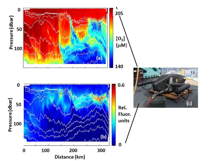
The Southern Ocean dominates the mean global ocean sink for anthropogenic carbon, but its sparse sampling relative to other basins limits our capacity to quantify carbon uptake and accompanying seasonal to interannual variability, which is critical to predicting future ocean carbon uptake and storage. Since 2002, underway pCO2 measurements collected as part of the Drake Passage Time-series (DPT) Program have informed our understanding of seasonally varying air-sea pCO2 gradients and by inference, the carbon fluxes in this region. Understanding whether Drake Passage air-sea fluxes are representative of the broader subpolar Southern Ocean was the focus of a recent study in Biogeosciences.
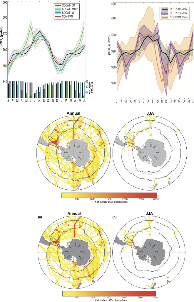
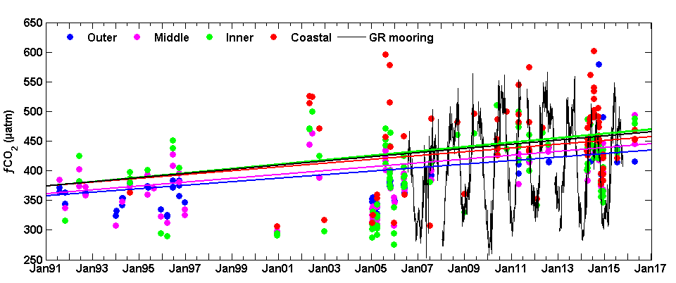
Top left panel: Mean surface ocean seasonal pCO2 cycle estimate for datasets from the Surface Ocean CO2 Atlas (SOCAT) in the subpolar Southern Ocean: black- SOCAT within the Drake Passage (DP) region; green- SOCAT outside the DP region; blue- all SOCAT in Southern Ocean Subpolar Seasonally Stratified (SPSS) biome; red- Self Organizing Map Feed-forward Network (SOM-FFN) product. Shading represents 1 standard error for biome-scale monthly means driven by interannual variability. Bar plot indicates the number of years containing observations in a given month (maximum of 15 years).
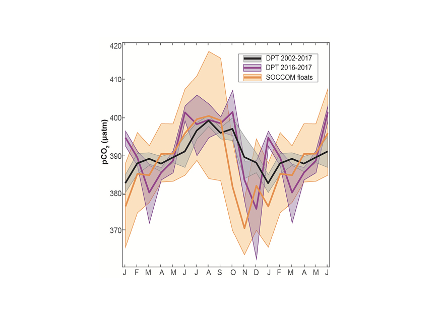
Top right panel: Mean surface ocean pCO2 seasonal cycle estimate for black: underway Drake Passage Time-series data for years 2002–2016; purple: DPT for years 2016–2017 to match years covered by the floats; and orange: SOCCOM floats. Seasonal cycles are shown on an 18-month cycle, calculated from a monthly mean time series with the atmospheric correction to year 2017. Shading represents 1 standard error accounting for the spatial and temporal heterogeneity of the sample and the measurement error (2.7 % or ±11 µatm at a pCO2 of 400 µatm for floats; ±2 µatm for DPT data) combined using the square root of the sum of squares.
An analysis of available Southern Ocean pCO2 data from inside vs. outside the Drake Passage showed agreement in the timing and amplitude of seasonal pCO2 variations, suggesting that the seasonality so carefully recorded by DPT is in fact representative of the broader subpolar Southern Ocean. DPT’s high temporal resolution sampling is critical to constraining estimates of the seasonal cycle of surface pCO2 in this region, as wintertime underway pCO2 data remain sparse outside the Drake Passage. Comparisons of the DPT data to an emerging dataset of float-estimated pCO2 from the SOCCOM (Southern Ocean Carbon and Climate Observations and Modeling) project showed that both shipboard and autonomous platforms capture the expected seasonal cycle for the subpolar Southern Ocean, with an austral wintertime peak driven by deep mixing and a summertime low driven by biological uptake. However, the seasonal cycle derived from float-estimated pCO2 has a larger seasonal amplitude compared to the DPT data due to an earlier and much lower observed summertime minimum.
The Drake Passage Time-series illustrates the large variability of surface ocean pCO2 in the Southern Ocean and exemplifies the value of sustained observations for understanding changing ocean carbon uptake in this dynamic region. Coordinated monitoring efforts that combine a robust ship-based observational network with a well-calibrated array of autonomous biogeochemical floats will improve and expand our understanding of the Southern Ocean carbon cycle in the future.
Authors:
Amanda R. Fay (Lamont Doherty Earth Observatory)
Nicole S. Lovenduski (University of Colorado)
Galen A. McKinley (Lamont Doherty Earth Observatory)
David R. Munro (University of Colorado)
Colm Sweeney (University of Colorado, NOAA Earth System Research Laboratory)
Alison R. Gray (University of Washington)
Peter Landschützer (Max Planck Institute for Meteorology, Germany)
Britton B. Stephens (National Center for Atmospheric Research)
Taro Takahashi (Lamont Doherty Earth Observatory)
Nancy Williams (Oregon State University)


