seasonal patterns :: Ocean Carbon & Biogeochemistry

Studying marine ecosystems and biogeochemical cycles in the face of environmental change

Archive for seasonal patterns

How atmospheric and oceanographic forcing impact the carbon sequestration in an ultra-oligotrophic marine system

Posted by mmaheigan

· Wednesday, August 11th, 2021

Sinking particles are a critical conduit for the export of material from the surface to the deep ocean. Despite their importance in oceanic carbon cycling, little is known about the composition and seasonal variability of sinking particles which reach abyssal depths. Oligotrophic waters cover ~75% of the ocean surface and contribute over 30% of the global marine carbon fixation. Understanding the processes that control carbon export to the deep oligotrophic areas is crucial to better characterize the strength and efficiency of the biological pump as well as to project the response of these systems to climate fluctuations and anthropogenic perturbations.

In a recent study published in Frontiers in Earth Science, authors synthesized data from atmospheric and oceanographic parameters, together with main mass components, and stable isotope and source-specific lipid biomarker composition of sinking particles collected in the deep Eastern Mediterranean Sea (4285m, Ierapetra Basin) for a three-year period (June 2010-June 2013). In addition, this study compared the sinking particulate flux data with previously reported deep-sea surface sediments from the study area to shed light on the benthic–pelagic coupling.

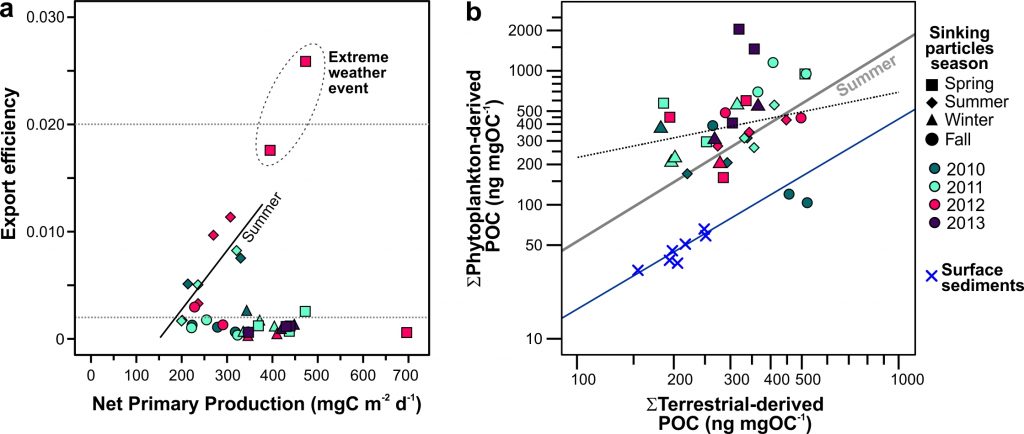
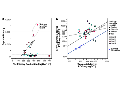
Figure Caption: a) Biplot of net primary productivity vs export efficiency (top and bottom horizontal dashed lines indicate threshold for high and low export efficiency regimes). b) Biplot of POC-normalized concentrations of terrestrial vs. phytoplankton-derived lipid biomarkers of the sinking particles collected in the deep Eastern Mediterranean Sea (Ierapetra Basin, NW Levantine Basin) from June 2010–June 2013, and surface sediments collected from January 2007 to June 2012 in the study area.

Both seasonal and episodic pulses are crucial for POC export to the deep Eastern Mediterranean Sea. POC fluxes peaked in spring April–May 2012 (12.2 mg m⁻² d⁻¹) related with extreme atmospheric forcing. Overall, summer particle export fuels more efficient carbon sequestration than the other seasons. The results of this study highlight that the combination of extreme weather events and aerosol deposition can trigger an influx of both marine labile carbon and anthropogenic compounds to the deep. Finally, the comparison of the sinking particles flux data with surface sediments revealed an isotopic discrimination, as well as a preferential degradation of labile organic matter during deposition and burial, along with higher preservation of land-derived POC in the underlying sediments. This study provides key knowledge to better understand the export, fate and preservation vs. degradation of organic carbon, and for modeling the organic carbon burial rates in the Mediterranean Sea.

Authors:
Rut Pedrosa-Pamies (The Ecosystems Center, Marine Biological Laboratory, US; Research Group in Marine Geosciences, University of Barcelona, Spain)
Constantine Parinos (Institute of Oceanography, Hellenic Centre for Marine Research, Greece)
Anna Sanchez-Vidal (Group in Marine Geosciences, University of Barcelona, Spain)
Antoni Calafat (Group in Marine Geosciences, University of Barcelona, Spain)
Miquel Canals (Group in Marine Geosciences, University of Barcelona, Spain)
Dimitris Velaoras (Institute of Oceanography, Hellenic Centre for Marine Research, Greece)
Nikolaos Mihalopoulos (Environmental Chemical Processes Laboratory, University of Crete; National Observatory of Athens, Greece)
Maria Kanakidou (Environmental Chemical Processes Laboratory, University of Crete Greece)
Nikolaos Lampadariou (Institute of Oceanography, Hellenic Centre for Marine Research, Greece)
Alexandra Gogou (Institute of Oceanography, Hellenic Centre for Marine Research, Greece)

Sea ice loss amplifies CO2 increase in the Arctic

Posted by mmaheigan

· Thursday, January 7th, 2021

Warming and sea ice loss over the past few decades have caused major changes in sea surface partial pressure of CO₂ (pCO₂) of the western Arctic Ocean, but detailed temporal variations and trends during this period of rapid climate-driven changes are not well known.

Based on an analysis of an international Arctic pCO₂ synthesis data set collected between 1994-2017, the authors of a recent paper published in Nature Climate Change observed that summer sea surface pCO₂ in the Canada Basin is increasing at twice the rate of atmospheric CO₂ rise. Warming, ice loss and subsequent CO₂ uptake in the Basin are amplifying seasonal pCO₂ changes, resulting in a rapid long-term increase. Consequently, the summer air-sea CO₂ gradient has decreased sharply and may approach zero by the 2030s, which is reducing the basin’s capacity to remove CO₂from the atmosphere. In stark contrast, sea surface pCO₂ on the Chukchi Shelf remains low and relatively constant during this time frame, which the authors attribute to increasingly strong biological production in response to higher intrusion of nutrient-rich Pacific Ocean water onto the shelf as a result of increased Bering Strait throughflow. These trends suggest that, unlike the Canada Basin, the Chukchi Shelf will become a larger carbon sink in the future, with implications for the deep ocean carbon cycle and ecosystem.

As Arctic sea ice melting accelerates, more fresh, low-buffer capacity, high-CO₂ water will enter the upper layer of the Canada Basin, which may rapidly acidify the surface water, endanger marine calcifying organisms, and disrupt ecosystem function.

Figure. 1: TOP) Sea surface pCO₂ trend in the Canada Basin and Chukchi Shelf. The grey dots represent the raw observations of pCO₂, black dots are the monthly mean of pCO₂ at in situ SST, and red dots are the monthly means of pCO₂ normalized to the long-term means of SST. The arrows indicate the statistically significant change in ∆pCO₂. BOTTOM) Sea ice-loss amplifying surface water pCO₂ in the Canada Basin. Black dots represent the initial condition for pCO₂ and DIC at -1.6 ℃. The arrows indicate the processes of warming (red), CO₂ uptake from the atmosphere (green), dilution by ice meltwater (blue). The yellow shaded areas indicate the possible seasonal variations of pCO₂, which are amplified by the synergistic effect of ice melt, warming and CO₂ uptake.

Authors:
Zhangxian Ouyang (University of Delaware, USA),
Di Qi (Third Institute of Oceanography, China),
Liqi Chen (Third Institute of Oceanography, China),
Taro Takahashi† (Columbia University, USA),
Wenli Zhong (Ocean University of China, China),
Michael D. DeGrandpre (University of Montana, USA),
Baoshan Chen (University of Delaware, USA),
Zhongyong Gao (Third Institute of Oceanography, China),
Shigeto Nishino (Japan Agency for Marine-Earth Science and Technology, Japan),
Akihiko Murata (Japan Agency for Marine-Earth Science and Technology, Japan),
Heng Sun (Third Institute of Oceanography, China),
Lisa L. Robbins (University of South Florida, USA),
Meibing Jin (International Arctic Research Center, USA),
Wei-Jun Cai* (University of Delaware, USA)

Water clarity impacts temperature and biogeochemistry in Chesapeake Bay

Posted by mmaheigan

· Thursday, December 3rd, 2020

Estuarine water clarity is determined by suspended materials in the water, including colored dissolved organic matter, phytoplankton, sediment, and detritus. These constituents directly affect temperature because when water is opaque, sunlight heats only the shallowest layers near the surface, but when water is clear, sunlight can penetrate deeper, warming the waters below the surface. Despite the importance of accurately predicting temperature variability, many numerical modeling studies do not adequately parameterize this fundamental relationship between water clarity and temperature.

In a recent study published in Estuaries and Coasts, the authors quantified the impact of a more realistic representation of water clarity in a hydrodynamic-biogeochemical model of the Chesapeake Bay by comparing two simulations: (1) water clarity is constant in space and time for the calculation of solar heating vs. (2) water clarity varies with modeled concentrations of light-attenuating materials. In the variable water clarity simulation (2), the water is more opaque, particularly in the northern region of the Bay. During the spring and summer months, the lower water clarity in the northern Bay is associated with warmer surface temperatures and colder bottom temperatures. Warmer surface temperatures encourage phytoplankton growth and nutrient uptake near the head of the Bay, thus fewer nutrients are transported downstream. These conditions are exacerbated during high-river flow years, when differences in temperature, nutrients, phytoplankton, and zooplankton extend further seaward.

Figure 1: Top row: Difference in the light attenuation coefficient for shortwave heating, kh[m-1] (variable minus constant light attenuation simulation). June, July, and August average for (A) 2001, (B) average of 2001-2005, and (C) 2003; difference in bottom temperatures [oC] (variable minus constant). Bottom row: Difference in June, July, and August average bottom temperature for (D) 2001, (E) average of 2001-2005, and (F) 2003. Data for 2001 are representative of low river discharge, and 2003 are representative high river discharge years.

This work demonstrates that a constant light attenuation scheme for heating calculations in coupled hydrodynamic-biogeochemical models underestimates temperature variability, both temporally and spatially. This is an important finding for researchers who use models to predict future temperature variability and associated impacts on biogeochemistry and species habitability.

Authors:
Grace E. Kim (NASA, Goddard Space Flight Center)
Pierre St-Laurent (VIMS, William & Mary)
Marjorie A.M. Friedrichs (VIMS, William & Mary)
Antonio Mannino (NASA, Goddard Space Flight Center)

Investigating variability and change in subpolar Southern Ocean pCO2 via time-series and float data

Posted by mmaheigan

· Tuesday, November 6th, 2018

The Southern Ocean dominates the mean global ocean sink for anthropogenic carbon, but its sparse sampling relative to other basins limits our capacity to quantify carbon uptake and accompanying seasonal to interannual variability, which is critical to predicting future ocean carbon uptake and storage. Since 2002, underway pCO₂measurements collected as part of the Drake Passage Time-series (DPT) Program have informed our understanding of seasonally varying air-sea pCO₂gradients and by inference, the carbon fluxes in this region. Understanding whether Drake Passage air-sea fluxes are representative of the broader subpolar Southern Ocean was the focus of a recent study in Biogeosciences.

Top left panel: Mean surface ocean seasonal pCO2 cycle estimate for datasets from the Surface Ocean CO2 Atlas (SOCAT) in the subpolar Southern Ocean: black- SOCAT within the Drake Passage (DP) region; green- SOCAT outside the DP region; blue- all SOCAT in Southern Ocean Subpolar Seasonally Stratified (SPSS) biome; red- Self Organizing Map Feed-forward Network (SOM-FFN) product. Shading represents 1 standard error for biome-scale monthly means driven by interannual variability. Bar plot indicates the number of years containing observations in a given month (maximum of 15 years).
Top right panel: Mean surface ocean pCO2 seasonal cycle estimate for black: underway Drake Passage Time-series data for years 2002–2016; purple: DPT for years 2016–2017 to match years covered by the floats; and orange: SOCCOM floats. Seasonal cycles are shown on an 18-month cycle, calculated from a monthly mean time series with the atmospheric correction to year 2017. Shading represents 1 standard error accounting for the spatial and temporal heterogeneity of the sample and the measurement error (2.7 % or ±11 µatm at a pCO2 of 400 µatm for floats; ±2 µatm for DPT data) combined using the square root of the sum of squares.

An analysis of available Southern Ocean pCO₂ data from inside vs. outside the Drake Passage showed agreement in the timing and amplitude of seasonal pCO₂ variations, suggesting that the seasonality so carefully recorded by DPT is in fact representative of the broader subpolar Southern Ocean. DPT’s high temporal resolution sampling is critical to constraining estimates of the seasonal cycle of surface pCO₂ in this region, as wintertime underway pCO₂ data remain sparse outside the Drake Passage. Comparisons of the DPT data to an emerging dataset of float-estimated pCO₂ from the SOCCOM (Southern Ocean Carbon and Climate Observations and Modeling) project showed that both shipboard and autonomous platforms capture the expected seasonal cycle for the subpolar Southern Ocean, with an austral wintertime peak driven by deep mixing and a summertime low driven by biological uptake. However, the seasonal cycle derived from float-estimated pCO₂ has a larger seasonal amplitude compared to the DPT data due to an earlier and much lower observed summertime minimum.

The Drake Passage Time-series illustrates the large variability of surface ocean pCO₂ in the Southern Ocean and exemplifies the value of sustained observations for understanding changing ocean carbon uptake in this dynamic region. Coordinated monitoring efforts that combine a robust ship-based observational network with a well-calibrated array of autonomous biogeochemical floats will improve and expand our understanding of the Southern Ocean carbon cycle in the future.

Authors:
Amanda R. Fay (Lamont Doherty Earth Observatory)
Nicole S. Lovenduski (University of Colorado)
Galen A. McKinley (Lamont Doherty Earth Observatory)
David R. Munro (University of Colorado)
Colm Sweeney (University of Colorado, NOAA Earth System Research Laboratory)
Alison R. Gray (University of Washington)
Peter Landschützer (Max Planck Institute for Meteorology, Germany)
Britton B. Stephens (National Center for Atmospheric Research)
Taro Takahashi (Lamont Doherty Earth Observatory)
Nancy Williams (Oregon State University)

Shelf-wide pCO2 increase across the South Atlantic Bight

Posted by mmaheigan

· Thursday, August 2nd, 2018

Relative to their surface area, coastal regions represent some of the largest carbon fluxes in the global ocean, driven by numerous physical, chemical and biological processes. Coastal systems also experience human impacts that affect carbon cycling, which has large socioeconomic implications. The highly dynamic nature of these systems necessitates observing approaches and numerical methods that can both capture high-frequency variability and delineate long-term trends.

Figure 1: The South Atlantic Bight (SAB) was divided into four sections using isobaths: the coastal zone (0 to 15 m), the inner shelf (15 to 30 m), the middle shelf (30 to 60 m), and the outer shelf (60 m and beyond). The X’s indicate the locations of the Gray’s Reef mooring (southern X) and the Edisto mooring (northern X).

In two recent studies using mooring- and ship-based ocean CO₂ system data, authors observed that pCO₂ is increasing from the coastal zone to the outer shelf of the South Atlantic Bight at rates greater than the global average oceanic and atmospheric increase (~1.8 µatm y^-1). In recent publications in Continental Shelf Research and JGR-Oceans, the authors analyzed pCO₂ data from 46 cruises (1991-2016) using a novel linear regression technique to remove the seasonal signal, revealing an increase in pCO₂ of 3.0-3.7 µatm y^-1on the outer and inner shelf, respectively. Using a Generalized Additive Mixed Model (GAMM) approach for trend analysis, authors observed that the rates of increase were slightly higher than the deseasonalization technique, yielding pCO₂ increases of 3.3 to 4.5 µatm y^-1 on the outer and inner shelf, respectively. The reported pCO₂ increases result in potential pH decreases of -0.003 to -0.004 units y^-1.

Figure 2: The time series of fCO2 in the four regions of the SAB (cruise observations) and from the Gray’s Reef mooring on the inner shelf indicate an increase across the shelf. These data are the observed values, however, the trend lines for each time series are calculated using deseasonalized values using the reference year method.

Analysis of the pCO₂ time-series from the Gray’s Reef mooring (using a NOAA Moored Autonomous pCO₂ system from July 2006 -July 2015) yielded a rate of increase (3.5 ± 0.9 µatm y^-1) that was comparable to the cruise data on the inner shelf (3.7 ± 2.2 and 4.5 ± 0.6 µatm y^-1, linear and GAMM methods, respectively). Validation data collected at the mooring suggest that underway data from cruises and the moored data are comparable. Neither thermal processes nor atmospheric dissolution (the primary driver of oceanic acidification) can explain the observed pCO₂ increase and concurrent pH decrease across the shelf. Unlike the middle and outer shelves, where an increase in SST could account for up to 1.1 µatm y^-1 of the observed pCO₂ trend, there is no thermal influence in the coastal zone and inner shelf. While 1.8 µatm y^-1 could be attributed to the global average atmospheric increase, the remainder is likely due to transport from coastal marshes and in situ biological processes. As the authors have shown, the increasing coastal and oceanic trend in pCO₂ can lead to a decrease in pH, especially if there is no increase in buffering capacity. More acidic waters can have a long term affect on coastal ecosystem services and biota.

Also see Eos Editor’s Vox on this research by Peter Brewer https://eos.org/editors-vox/coastal-ocean-warming-adds-to-co2-burden

Authors:

Multidecadal fCO2 Increase Along the United States Southeast Coastal Margin (JGR-Oceans)
Janet J. Reimer (University of Delaware)
Hongjie Wang (Texas A &M University – Corpus Christi)
Rodrigo Vargas (University of Delaware)
Wei-Jun Cai (University of Delaware)

And

Time series pCO2 at a coastal mooring: Internal consistency, seasonal cycles, and interannual variability (Continental Shelf Research)
Janet J. Reimer (University of Delaware)
Wei-Jun Cai (University of Delaware; University of Georgia)
Liang Xue (University of Delaware; First Institute of Oceanography, China)
Rodrigo Vargas (University of Delaware)
Scott Noakes (University of Georgia)
Xinping Hu (Texas A &M University – Corpus Christi)
Sergio R. Signorini (Science Applications International Corporation)
Jeremy T. Mathis (NOAA Arctic Research Program)
Richard A. Feely (NOAA Pacific Marine Environmental Laboratory)
Adrienne J. Sutton (NOAA Pacific Marine Environmental Laboratory; University of Washington)
Christopher Sabine (University of Hawaii Manoa)
Sylvia Musielewicz (NOAA Pacific Marine Environmental Laboratory; University of Washington)
Baoshan Chen (University of Delaware; University of Georgia)
Rik Wanninkhof (NOAA Atlantic Oceanographic and Meteorological Laboratory)

Untangling the mystery of domoic acid events: A climate-scale perspective

Posted by mmaheigan

· Thursday, August 3rd, 2017

The diatom Pseudo-nitzchia produces a neurotoxin called domoic acid, which in high concentrations affects wildlife ranging from mussels and crabs to seabirds and sea lions, as well as humans. In humans, the effects of domoic acid poisoning can range from gastrointestinal distress to memory loss, and even death. Despite being studied in laboratories since the late 1980s, there is no consensus on the environmental conditions that lead to domoic acid events. These events are most frequent and impactful in eastern boundary current regions such as the California Current System, which is bordered by Washington, Oregon, and California. In Oregon alone, there have been six major domoic acid events: 1996, 1998-1999, 2001, 2002-2006, 2010, 2014-2015. McKibben et al. (2017) investigated the regulation of domoic acid at a climate scale to develop and test an applied risk model for the US West Coast” to read “McKibben et al. (2017) investigated the regulation of domoic acid at regional and decadal scales in order to develop and test an applied risk model for the impact of climate on the US West Coast. They used the PDO and ONI climate variability indices, averages of monthly and 3 month running means of SST anomaly values and variability to look at basin-scale ocean conditions. At a local scale, data were from zooplankton sampling every two to four weeks between 1996 to 2015 at hydrographic station offshore of Newport, OR. Additionally, the NOAA NCDC product “Daily Optimum Interpolation, Advanced Very High Resolution Radiometer Only, Version 2, Final+Preliminary SST” was used to obtain the monthly SST anomaly metric, based on combined in situ and satellite data.

(A) Warm and cool ocean regimes, (B) local SST anomaly, and (C and D) biological response. (A) PDO (red or blue vertical bars) and ONI (black line) indices; strong (S) to moderate (M) El Nino (+1) and La Nina (−1) events are labeled. (B) SST anomaly 20 nm off central OR. (C) The CSR anomaly 5 nm off central OR. (D) Monthly OR coastal maximum DA levels in razor clams (vertical bars); horizontal black line is the 20-ppm closure threshold. Black line in D shows the spring biological transition date (right y axis). At the top of the figure, black boxes indicate the duration of upwelling season each year; red vertical bars indicate the timing of annual DA maxima in relationship to upwelling. Gray shaded regions are warm regimes based on the PDO. Dashed vertical lines indicate onset of the six major DA events. The September 2014 arrival of the NE Pacific Warm Anomaly (colloquially termed “The Blob”) to the OR coastal region is labeled on B. “X” symbols along the x axes indicate that no data were available for that month (B–D).

Their findings show that these events have occurred when there is advection of warmer water masses onto the continental shelf from southern or offshore areas. When the warm phase of the Pacific Decadal Oscillation (PDO) and El Niño coincide, the effect is additive. In the warm regime years, there is a later spring biological transition date, weaker alongshore currents, elevated water temperatures, and plankton communities are dominated by subtropical rather than subarctic species. The authors also note relative differences between the prevalence and phenology of domoic acid events in OR, CA and WA, which warrants further study via regional-scale modeling. Overall, this research shows a clear and enhanced risk of toxicity in shellfish during warm phases of natural climate oscillations. If predictions of more extreme warming come to bear, this would potentially lead to increased DA event intensity and frequency in coastal zones around the globe. This will not only affect wildlife, but may cause significant closures of economically important fisheries (e.g., Dungeness crab, anchovy, mussel, and razor clam), which would impact local communities and native populations.

Authors:
Morgaine McKibben (Oregon State Univ., NOAA Northwest Fisheries Science Center)
William Peterson (NOAA Northwest Fisheries Science Center)
Michelle Wood (Univ. Oregon)
Vera L. Trainer (NOAA Northwest Fisheries Science Center)
Matthew Hunter (Oregon Dept. Fish & Wildlife)
Angelicque E. White (Oregon State Univ.)

Winter ventilation depth constrains the impact of the biological pump on CO2 uptake in the North Pacific Ocean

Posted by mmaheigan

· Thursday, June 8th, 2017

The North Pacific accounts for ~25% of the global ocean’s uptake of carbon dioxide (CO₂) from the atmosphere. However, the relative importance of the biological pump vs. physical circulation in driving ocean uptake of CO₂ remains poorly understood.

In a recent study, Palevsky and Quay (2017) used geochemical measurements collected on sixteen container ship transects between Hong Kong and Long Beach, CA to evaluate the drivers of CO₂ uptake across 8,000 kilometers in the North Pacific basin over the full annual cycle. In the eastern North Pacific, biologically-driven export of organic carbon below the winter ventilation depth fully offsets the uptake of CO₂ from the atmosphere. However, in the Kuroshio region of the western North Pacific, which has a deep winter mixed layer, the majority of the organic carbon exported during the productive summer season is subsequently respired and ventilated back to the atmosphere in winter. Subsequently, biologically-driven export offsets only a small fraction of the CO₂ uptake by the ocean and, instead, physical transport is the dominant process removing inorganic carbon from the region.

We further show that that mechanistic coupling between biological carbon export and ocean uptake of CO₂ from the atmosphere is sensitive to the seasonal timing of biological export and ventilation, as well as the magnitude of export. Future studies therefore need to measure biological carbon export and ventilation throughout the full annual cycle in order to better understand controls on regional variations in ocean CO₂ uptake rates and future changes in these rates.

Data from 16 shipboard transects across the North Pacific revealed a basin-wide gradient between the Kuroshio and Eastern regions in the relative roles of biological vs. physical processes in removing dissolved inorganic carbon from the surface ocean.

Authors:
Hilary I. Palevsky (Woods Hole Oceanographic Institution)
Paul D. Quay (University of Washington)

Scientists reveal major drivers of aragonite saturation state in the Gulf of Maine, a region vulnerable to acidification

Posted by mmaheigan

· Thursday, May 11th, 2017

The Gulf of Maine (GoME) is a shelf region that is especially vulnerable to ocean acidification (OA). GoME’s shelf waters display the lowest mean pH, aragonite saturation state (Ω-Ar), and buffering capacity of the entire U.S. East Coast. These conditions are a product of many unique characteristics and processes occurring in the GoME, including relatively low water temperatures that result in higher CO₂ solubility; inputs of fresher, low-alkalinity water that is traceable to the rivers discharging into the Labrador Sea to the north, as well as local inputs of low-pH river water; and its semi-enclosed nature (long residence time >1 year), which enables the accumulation of respiratory products, i.e. CO₂.

A recent study by Wang et al. (2017) is the first to assess the major oceanic processes controlling seasonal variability of aragonite saturation state and its linkages with pteropod abundance in the GoME. The results indicate that surface production was tightly coupled with remineralization in the benthic nepheloid layer during highly productive seasons, resulting in occasional aragonite undersaturation. Mean water column Ω-Ar and abundance of large thecosomatous pteropods show some correlation, although discrete cohort reproductive success likely also influences their abundance. Photosynthesis-respiration is the primary driving force controlling Ω-Ar variability over the seasonal cycle. However, calcium carbonate (CaCO₃) dissolution appears to occur at depth in fall and winter months when bottom water Ω-Ar is generally low but slightly above 1. This is accompanied by a decrease in pteropod abundance that is consistent with previous CaCO₃ flux trap measurements.

Figure. Changes of aragonite saturation states (ΔΩ) between three consecutive cruises from April – July 2015 as a function of changes in salinity-normalized DIC (ΔenDIC, including correction of freshwater inputs) (a) and changes in salinity-normalized TA (ΔenTA, including correction of freshwater inputs) (b). The data points circled in (b) represent potential alkalinity sources from CaCO3 dissolution and/or anaerobic respiration. Solid lines are theoretical lines of ΔΩ vs. ΔenDIC and ΔΩ vs. ΔenTA expected if only photosynthesis and respiration/remineralization occur. Dashed lines are theoretical lines if only calcification and dissolution of CaCO3 occur.

Under the current rate of OA, the mean Ω-Ar of the subsurface and bottom waters of the GoME will approach undersaturation (Ω-Ar < 1) in 30-40 years. As photosynthesis and respiration are the major driving mechanisms of Ω-Ar variability in the water column, any biological regime changes may significantly impact carbonate chemistry and the GoME ecosystem, including the CaCO₃ shell-building capacity of organisms that are critical to the GoME food web.

Author:

Zhaohui Aleck Wang (Woods Hole Oceanographic Institution)

Satellite Laser Lights Up Polar Research

Posted by mmaheigan

· Thursday, April 13th, 2017

What controls annual cycles and interannual changes in polar phytoplankton biomass? Answers to this question are now emerging from a satellite light detection and ranging (lidar) sensor, which can observe the polar oceans throughout the extensive periods when measurements from traditional passive ocean color sensors are impossible. The new study uses active lidar measurements from the CALIOP satellite sensor to construct complete decade-long record of phytoplankton biomass in the northern and southern polar regions. Results of the study show that annual cycles in biomass are driven by rates of acceleration and deceleration in phytoplankton division, with bloom termination coinciding with maximum division rates irrespective of whether nutrients are exhausted. The study further shows that interannual differences in bloom strength can be quantitatively related to the difference between the winter minimum to summer maximum in division rates. Finally, the analysis indicated that ecological processes had a greater impact than ice cover changes on integrated polar zone phytoplankton biomass in the north, whereas ice cover changes were the dominant driver in the south polar zone. Despite being designed for atmospheric research, CALIOP has provided the first demonstration that active satellite lidar measurements can yield important new insights on plankton ecology in the climate sensitive polar regions. This proof-of-concept creates a foundation for a future ocean-optimized sensor with water-column profiling capabilities that would launch a new lidar era in satellite oceanography.

Authors:

Michael J. Behrenfeld (Oregon State Univ.)
Yongxiang Hu (NASA Langley Research Center)
Robert T. O’Malley (Oregon State Univ.)
Emmanuel S. Boss (Univ. Maine)
Chris A. Hostetler (NASA Langley Research Center)
David A. Siegel (Univ. California Santa Barbara)
Jorge Sarmiento (Princeton Univ.)
Jennifer Schulien (Oregon State Univ.)
Johnathan W. Hair (NASA Langley Research Center)
Xiaomei Lu (NASA Langley Research Center)
Sharon Rodier (NASA Langley Research Center)
Amy Jo Scarino (NASA Langley Research Center)

A framework for ENSO predictability of marine ecosystem drivers along the US West Coast

Posted by mmaheigan

· Thursday, February 16th, 2017

The US West Coast eastern boundary upwelling system supports one of the most productive marine ecosystems in the world and is a primary source of ecosystem services for the US (e.g., fishing, shipping, and recreation). Long-term historical observations of physical and biological variables in this region have been collected since the 1950s (e.g., the CalCOFI program and now including the coastal ocean observing systems), leading to an excellent foundation for understanding the ecosystem impacts of dominant climate fluctuations such as the El Niño-Southern Oscillation (ENSO). In the northeast Pacific, ENSO impacts a wide range of physical and biotic processes, including temperature, stratification, winds, upwelling, and primary and secondary production. The El Niño phase of ENSO, in particular, can result in extensive geographic habitat range displacements and altered catches of fishes and invertebrates, and impact vertical and lateral export fluxes of carbon and other elements (Jacox et al., this issue; Anderson et al., this issue; Ohman et al., this issue). However, despite empirical observations and increased understanding of the coupling between climate and marine ecosystems along the US West Coast, there has been no systematic attempt to use this knowledge to forecast marine ecosystem responses to individual ENSO events. ENSO forecasting has become routine in the climate community. However, little has been done to forecast the impacts of ENSO on ecosystems and their services. This becomes especially important considering the occurrence of recent strong El Niño events (such as 2015-16) and climate model projections that suggest that ENSO extremes may become more frequent (Cai et al. 2015).

The joint US CLIVAR/OCB/NOAA/PICES/ICES workshop on Forecasting ENSO impacts on marine ecosystems of the US West Coast (Di Lorenzo et al. 2017) held in La Jolla, California, in August 2016 outlined a three-step strategy to better understand and quantify the ENSO-related predictability of marine ecosystem drivers along the US West Coast (Figure 1). The first step is to use a high-resolution ocean reanalysis to determine the association between local ecosystem drivers and regional forcing patterns (RFPs). The identification of ecosystem drivers will depend on the ecosystem indicators or target species selected for prediction (Ohman et al., this issue). The second step is to objectively identify the tropical sea surface temperature (SST) patterns that optimally force the RFPs along the US West Coast region using available long-term large-scale reanalysis products. While the goal of the first two steps is to understand the dynamical basis for predictability (Figure 1, blue path), the final third step (Figure 1, orange path) aims at quantifying the predictability of the RFPs and estimating their prediction skill at seasonal timescales. This third step can be implemented using the output of multi-model ensemble forecasts such as the North America Multi-Model Ensemble (NMME) or by building efficient statistical prediction models such as Linear Inverse Models (LIMs; Newman et al. 2003).

Figure 1. Framework for understanding and predicting ENSO impacts on ecosystem drivers. Blue path shows the steps that will lead to Understanding of the ecosystem drivers and their dependence on tropical Pacific anomalies. Orange path shows the steps that will lead to quantifying the Predictability of marine ecosystem drivers along the US West Coast that are predictable from large-scale tropical teleconnection dynamics.

Important to the concept of ENSO predictability is the realization that the expressions of ENSO are very diverse and cannot be identified with a few indices (Capotondi et al. 2015; Capotondi et al., this issue). In fact, different expressions of sea surface temperature anomalies (SSTa) in the tropics give rise to oceanic and atmospheric teleconnections that generate different coastal impacts in the northeast Pacific. For this reason, we will refer to ENSO as the collection of tropical Pacific SSTa that lead to deterministic and predictable responses in the regional ocean and atmosphere along the US West Coast.

In the sections below, we articulate in more detail the elements of the framework for quantifying the predictability of ENSO-related impacts on coastal ecosystems along the US West Coast (Figure 1). Our focus will be on the California Current System (CCS), reflecting the regional expertise of the workshop participants. Specifically, we discuss (1) the ecosystem drivers and what is identified as such; (2) RFP definitions; and (3) the teleconnections from the tropical Pacific and their predictability.

Ecosystem drivers in the California Current System

The impacts of oceanic processes on the CCS marine ecosystem have been investigated since the 1950s when the long-term California Cooperative Oceanic Fisheries Investigations (CalCOFI) began routine seasonal sampling of coastal ocean waters. The CalCOFI program continues today and has been augmented with several other sampling programs (e.g., the coastal ocean observing network), leading to an unprecedented understanding of how climate and physical ocean processes, such as upwelling, drive ecosystem variability and change (e.g., see more recent reviews from King et al.2011; Ohman et al. 2013; Di Lorenzo et al. 2013).

The dominant physical oceanographic drivers of ecosystem variability occur on seasonal, interannual, and decadal timescales and are associated with changes in (1) SST; (2) upwelling velocity; (3) alongshore transport; (4) cross-shore transport; and (5) thermocline/nutricline depth (see Ohman et al., this issue). This set of ecosystem drivers emerged from discussions among experts at the workshop. Ecosystem responses to these drivers include multiple trophic levels, including phytoplankton, zooplankton, small pelagic fish, and top predators, and several examples have been identified for the CCS (see summary table in Ohman et al., this issue).

While much research has focused on diagnosing the mechanisms by which these physical drivers impact marine ecosystems, less is known about the dynamics controlling the predictability of these drivers. As highlighted in Ohman et al. (this issue), most of the regional oceanographic drivers (e.g., changes in local SST, upwelling, transport, thermocline depth) are connected to changes in large-scale forcings (e.g., winds, surface heat fluxes, large-scale SST and sea surface height patterns, freshwater fluxes, and remotely forced coastally trapped waves entering the CCS from the south). In fact, several studies have documented how large-scale changes in wind patterns associated with the Aleutian Low and the North Pacific Oscillation drive oceanic modes of variability such as the Pacific Decadal Oscillation and the North Pacific Gyre Oscillation (Mantua et al. 1997; Di Lorenzo et al. 2008; Chhak et al. 2009; Ohman et al., this issue; Jacox et al., this issue; Anderson et al., this issue; Capotondi et al., this issue) that influence the CCS. However, these large-scale modes only explain a fraction of the ecosystem’s atmospheric forcing functions at the regional-scale. Thus, it is important to identify other key forcings to gain a more complete mechanistic understanding of CCS ecosystem drivers (e.g., Jacox et al. 2014; 2015).

Atmospheric and oceanic regional forcing patterns

The dominant large-scale quantities that control the CCS ecosystem drivers are winds, heat fluxes, and remotely forced coastally trapped waves (Hickey 1979). Regional expressions or patterns of these large-scale forcings have been linked to changes in local stratification and thermocline depth (Veneziani et al. 2009a; 2009b; Combes et al. 2013), cross-shore transport associated with mesoscale eddies (Kurian et al. 2011; Todd et al. 2012; Song et al. 2012; Davis and Di Lorenzo 2015b), and along-shore transport (Davis and Di Lorenzo 2015a; Bograd et al. 2015). For this reason, we define the regional expressions of the atmospheric and remote wave forcing that are optimal in driving SST, ocean transport, upwelling, and thermocline depth as the RFPs. To clarify this concept, consider the estimation of coastal upwelling velocities. While a change in the position and strength in the Aleutian Low has been related to coastal upwelling in the northern CCS, a more targeted measure of the actual upwelling vertical velocity and nutrient fluxes that are relevant to primary productivity can only be quantified by taking into account a combination of oceanic processes that depend on multiple RFPs such as thermocline depth (e.g., remote waves), thermal stratification (e.g., heat fluxes), mesoscale eddies, and upwelling velocities (e.g., local patterns of wind stress curl and alongshore winds; see Gruber et al 2011; Jacox et al. 2015; Renault et al. 2016). In other words, if we consider the vertical coastal upwelling velocity (w) along the northern CCS, a more adequate physical description and quantification would be given from a linear combination of the different regional forcing functions w = Σ_n∝_n * RFP_n rather than w = ∝*Aleutian Low.

The largest interannual variability in the Pacific that impacts the RFPs is ENSO, which also constitutes the largest source of seasonal (3-6 months) predictability. During El Niño and La Niña, atmospheric and oceanic teleconnections from the tropics modify large-scale and local surface wind patterns and ocean currents of the CCS and force coastally trapped waves.

ENSO teleconnections and potential seasonal predictability of the regional forcing patterns

While ENSO exerts important controls on the RFPs in the CCS, it has become evident that ENSO expressions in the tropics vary significantly from event to event, leading to different responses in the CCS (Capotondi et al., this issue). Also, as previously pointed out, the CCS is not only sensitive to strong ENSO events but more generally responds to a wide range of tropical SSTa variability that is driven by ENSO-type dynamics in the tropical and sub-tropical Pacific. For this reason, we define an “ENSO teleconnection” as any RFP response that is linked to ENSO-type variability in the tropics.

ENSO can influence the upwelling and circulation in the CCS region through both oceanic and atmospheric pathways. It is well known that equatorial Kelvin waves, an integral part of ENSO dynamics, propagate eastward along the Equator and continue both northward (and southward) along the coasts of the Americas as coastally trapped Kelvin waves after reaching the eastern ocean boundary. El Niño events are associated with downwelling Kelvin waves, leading to a deepening of the thermocline, while La Niña events produce a shoaling of the thermocline in the CCS (Simpson 1984; Lynn and Bograd 2002; Huyer et al. 2002; Bograd et al. 2009; Hermann et al. 2009; Miller et al. 2015). The offshore scale of coastal Kelvin waves decreases with latitude, and the waves decay while propagating northward along the coast due to dissipation and radiation of westward propagating Rossby waves. In addition, topography and bathymetry can modify the nature of the waves and perhaps partially impede their propagation at some location. Thus, the efficiency of coastal waves of equatorial origin in modifying the stratification in the CCS is still a matter of debate. To complicate matters, regional wind variability south of the CCS also excites coastally trapped waves, which supplement the tropical source.

In the tropics, SST anomalies associated with ENSO change tropical convection and excite mid-troposphere stationary atmospheric Rossby waves that propagate signals to the extratropics, the so-called atmospheric ENSO teleconnections (Capotondi et al., this issue). Through these atmospheric waves, warm ENSO events favor a deepening and southward shift of the Aleutian Low pressure system that is dominant during winter, as well as changes in the North Pacific Subtropical High that is dominant during spring and summer, resulting in a weakening of the alongshore winds, reduced upwelling, and warmer surface water. These changes are similar to those induced by coastal Kelvin waves of equatorial origin, making it very difficult to distinguish the relative importance of the oceanic and atmospheric pathways in the CCS. In addition, due to internal atmospheric noise, the details of the ENSO teleconnections can vary significantly from event to event and result in important differences along the California Coast (Figure 2).

Figure 2. Schematic of ENSO teleconnection associated with different flavors of tropical SSTa. (a) Atmospheric teleconnections of the canonical eastern Pacific El Niño tend to impact the winter expression of the Aleutian Low, which in turn drives an oceanic SSTa anomaly that projects onto the pattern of the Pacific Decadal Oscillation (PDO). (b) Atmospheric teleconnections of the central Pacific El Niño tend to impact the winter expression of the North Pacific High, which in turn drives an oceanic SSTa anomaly that projects onto the pattern of the North Pacific Gyre Oscillation (NPGO). The ENSO SSTa maps are obtained by regressing indices of central and eastern Pacific ENSO with SSTa. The other maps are obtained by regression of SSTa/SLPa with the PDO (a) and NPGO (b) indices.

El Niño events exhibit a large diversity in amplitude, duration, and spatial pattern (Capotondi et al. 2015). The amplitude and location of the maximum SST anomalies, whether in the eastern (EP) or central (CP) Pacific, can have a large impact on ENSO teleconnections (Ashok et al. 2007; Larkin and Harrison 2005). While “canonical” EP events induce changes in the Aleutian Low (Figure 2b), CP events have been associated with a strengthening of the second mode of North Pacific atmospheric variability, the North Pacific Oscillation (NPO; Figure 2a; Di Lorenzo et al. 2010; Furtado et al. 2012). In addition, it is conceivable that EP events have a larger Kelvin wave signature than CP events, resulting in different oceanic influences in the CCS.

In summary, while the ENSO influence on the CCS physical and biological environments is undeniable, several sources of uncertainty remain about the details of that influence. This uncertainty arises in the physical environment on seasonal timescales from many sources, including the diversity of ENSO events, the intrinsic unpredictable components of the atmosphere, and the intrinsic unpredictable eddy variations in the CCS. We also need to distinguish between physically forced ecosystem response versus intrinsic biological variability, which is potentially nonlinear and likely unpredictable. Skill levels need to be quantified for each step of the prediction process (i.e., ENSO, teleconnections, local oceanic response, local ecosystem response) relative to a baseline—for example the persistence of initial condition, which is also being exploited for skillful predictions of the large marine ecosystem at the seasonal timescale (Tommasi et al., this issue). The target populations should be exploitable species that are of interest to federal and state agencies that regulate certain stocks. Models are currently being developed to use ocean forecasts to advance top predator management (Hazen et al., this issue). The implementation of this framework (Figure 1) for practical uses will require a collaborative effort between physical climate scientists with expertise in predicting and understanding ENSO and biologists who have expertise in understanding ecosystem response to physical climate forcing.

Authors

Emanuele Di Lorenzo (Georgia Institute of Technology)
Arthur J. Miller (Scripps Institution of Oceanography)

References

Ashok, K., S.K. Behera, S.A. Rao, H. Weng, and T. Yamagata, 2007: El Niño Modoki and its possible teleconnections. J. Geophys. Res., 112, doi:10.1029/2006JC003798

Bograd, S. J., M. Pozo Buil, E. Di Lorenzo, C. G. Castro, I. D. Schroeder, R. Goericke, C. R. Anderson, C. Benitez-Nelson, and F. A. Whitney, 2015: Changes in source waters to the Southern California Bight. Deep-Sea Res. Part II-Top. Stud. Oceanogr., 112, 42-52, doi:10.1016/j.dsr2.2014.04.009.

Bograd, S. J., I. Schroeder, N. Sarkar, X. Qiu, W. J. Sydeman, and F. B. Schwing, 2009: Phenology of coastal upwelling in the California Current. Geophy. Res. Lett., 36, doi: 10.1029/2008GL035933.

Cai, W. J., and Coauthors, 2015: ENSO and greenhouse warming. Nature Climate Change, 5, 849-859, doi:10.1038/nclimate2743.

Capotondi, A., and Coauthors, 2015: Understanding ENSO Diversity. Bull. Amer. Meteor. Soc., 96, 921-938, doi:10.1175/BAMS-D-13-00117.1.

Chhak, K. C., E. Di Lorenzo, N. Schneider, and P. F. Cummins, 2009: Forcing of low-frequency ocean variability in the northeast Pacific. J. Climate, 22, 1255-1276, doi:10.1175/2008jcli2639.1.

Davis, A., and E. Di Lorenzo, 2015a: Interannual forcing mechanisms of California Current transports I: Meridional Currents. Deep-Sea Res. Part II-Top. Stud. Oceanogr., 112, 18-30, doi:10.1016/j.dsr2.2014.02.005.

Davis, A., and E. Di Lorenzo, 2015b: Interannual forcing mechanisms of California Current transports II: Mesoscale eddies. Deep-Sea Res. Part II-Top. Stud. Oceanogr., 112, 31-41, doi:10.1016/j.dsr2.2014.02.004.

Di Lorenzo, E., and Coauthors, 2017: Forecasting ENSO impacts on marine ecosystems of the US West Coast, Joint US CLIVAR/NOAA/PICES/ICES Report, https://usclivar.org/meetings/2016-enso-ecosystems, forthcoming.

Di Lorenzo, E., and Coauthors, 2008: North Pacific Gyre Oscillation links ocean climate and ecosystem change. Geophys. Res. Lett., 35, doi:10.1029/2007gl032838.

Di Lorenzo, E., and Coauthors, 2013: Synthesis of Pacific Ocean climate and ecosystem dynamics. Oceanogr., 26, 68-81, doi: 10.5670/oceanog.2013.76.

Di Lorenzo, E., K. M. Cobb, J. C. Furtado, N. Schneider, B. T. Anderson, A. Bracco, M. A. Alexander, and D. J. Vimont, 2010: Central Pacific El Nino and decadal climate change in the North Pacific Ocean. Nature Geosci., 3, 762-765, doi:10.1038/ngeo984.

Furtado, J. C., E. Di Lorenzo, B. T. Anderson, and N. Schneider, 2012: Linkages between the North Pacific Oscillation and central tropical Pacific SSTs at low frequencies. Climate Dyn., 39, 2833-2846, doi:10.1007/s00382-011-1245-4.

Gruber, N., Z. Lachkar, H. Frenzel, P. Marchesiello, M. Munnich, J. C. McWilliams, T. Nagai, and G. K. Plattner, 2011: Eddy-induced reduction of biological production in eastern boundary upwelling systems. Nature Geosci., 4, 787-792, doi:10.1038/ngeo1273.

Hermann, A. J., E. N. Curchitser, D. B. Haidvogel, and E. L. Dobbins, 2009: A comparison of remote vs. local influence of El Nino on the coastal circulation of the northeast Pacific. Deep Sea Res. Part II: Top. Stud. Oceanogr., 56, 2427-2443, doi: 10.1016/j.dsr2.2009.02.005.

Hickey, B. M., 1979. The California Current system—hypotheses and facts. Prog. Oceanogr., 8, 191-279, doi: 10.1016/0079-6611(79)90002-8.

Huyer, A., R. L. Smith, and J. Fleischbein, 2002: The coastal ocean off Oregon and northern California during the 1997–8 El Nino. Prog. Oceanogr., 54, 311-341, doi: 10.1016/S0079-6611(02)00056-3.

Jacox, M. G., A. M. Moore, C. A. Edwards, and J. Fiechter, 2014: Spatially resolved upwelling in the California Current System and its connections to climate variability. Geophy. Res. Lett., 41, 3189-3196, doi:10.1002/2014gl059589.

Jacox, M. G., J. Fiechter, A. M. Moore, and C. A. Edwards, 2015: ENSO and the California Current coastal upwelling response. J. Geophy. Res.-Oceans, 120, 1691-1702, doi:10.1002/2014jc010650.

Jacox, M. G., S. J. Bograd, E. L. Hazen, and J. Fiechter, 2015: Sensitivity of the California Current nutrient supply to wind, heat, and remote ocean forcing. Geophys. Res. Lett., 42, 5950-5957, doi:10.1002/2015GL065147.

Jacox, M. G., E. L. Hazen, K. D. Zaba, D. L. Rudnick, C. A. Edwards, A. M. Moore, and S. J. Bograd, 2016: Impacts of the 2015-2016 El Niño on the California Current System: Early assessment and comparison to past events. Geophys. Res. Lett., 43, 7072-7080, doi:10.1002/2016GL069716.

King, J. R., V. N. Agostini, C. J. Harvey, G. A. McFarlane, M. G. G. Foreman, J. E. Overland, E. Di Lorenzo, N. A. Bond, and K. Y. Aydin, 2011: Climate forcing and the California Current ecosystem. Ices J. Mar. Sci., 68, 1199-1216, doi:10.1093/icesjms/fsr009.

Kurian, J., F. Colas, X. Capet, J. C. McWilliams, and D. B. Chelton, 2011: Eddy properties in the California Current System. J. Geophy. Res.-Oceans, 116, doi:10.1029/2010jc006895.

Larkin, N. K. and D. E. Harrison, 2005: On the definition of El Niño and associated seasonal average US weather anomalies. Geophy. Res. Lett. 32, doi: 10.1029/2005GL022738.

Lynn, R. J. and S. J. Bograd, 2002: Dynamic evolution of the 1997–1999 El Niño–La Niña cycle in the southern California Current system. Prog. Oceanogr., 54, 59-75, doi: 10.1016/S0079-6611(02)00043-5.

Mantua, N. J., S. R. Hare, Y. Zhang, J. M. Wallace, and R. C. Francis, 1997: A Pacific interdecadal climate oscillation with impacts on salmon production. Bull. Amer. Meteorol. Soc., 78, 1069-1079, doi:10.1175/1520-0477(1997)078<1069:apicow>2.0.co;2.

Marchesiello, P., J. C. McWilliams, and A. Shchepetkin, 2003: Equilibrium structure and dynamics of the California Current System. J. Phys. Oceanogr., 33, 753-783, doi: 10.1175/1520-0485(2003)33<753:ESADOT>2.0.CO;2.

McCreary, J. P., P. K. Kundu, and S. Y. Chao, 1987: On the dynamics of the California Current System. J. Mar. Res., 45, 1-32, doi: 10.1357/002224087788400945.

Miller, A. J., H. Song, and A. C. Subramanian, 2015: The physical oceanographic environment during the CCE-LTER Years: Changes in climate and concepts. Deep Sea Res. Part II: Top. Stud. Oceanogr., 112, 6-17, doi: 10.1016/j.dsr2.2014.01.003.

Newman, M., and Coauthors, 2016: The Pacific Decadal Oscillation, Revisited. J. Climate, 29, 4399-4427, doi:10.1175/jcli-d-15-0508.1.

Ohman, M. D., K. Barbeau, P. J. S. Franks, R. Goericke, M. R. Landry, and A. J. Miller, 2013: Ecological transitions in a coastal upwelling ecosystem. Oceanogr., 26, 210-219, doi: 10.5670/oceanog.2013.65.

Renault, L., C. Deutsch, J. C. McWilliams, H. Frenzel, J.-H. Liang, and F. Colas, 2016: Partial decoupling of primary productivity from upwelling in the California Current system. Nature Geosci, 9, 505-508, doi:10.1038/ngeo2722.

Simpson, J. J., 1984; El Nino‐induced onshore transport in the California Current during 1982‐1983. Geophy. Res. Lett., 11, 233-236, doi: 10.1029/GL011i003p00233.

Song, H., A. J. Miller, B. D. Cornuelle, and E. Di Lorenzo, 2011: Changes in upwelling and its water sources in the California Current System driven by different wind forcing. Dyn. Atmos. Oceans, 52, 170-191, doi:10.1016/j.dynatmoce.2011.03.001.

Todd, R. E., D. L. Rudnick, M. R. Mazloff, B. D. Cornuelle, and R. E. Davis, 2012: Thermohaline structure in the California Current System: Observations and modeling of spice variance. J. Geophy. Res.-Oceans, 117, doi:10.1029/2011jc007589.

Veneziani, M., C. A. Edwards, J. D. Doyle, and D. Foley, 2009: A central California coastal ocean modeling study: 1. Forward model and the influence of realistic versus climatological forcing. J. Geophy. Res.-Oceans, 114, doi:10.1029/2008jc004774.

Veneziani, M., C. A. Edwards, and A. M. Moore, 2009: A central California coastal ocean modeling study: 2. Adjoint sensitivities to local and remote forcing mechanisms. J. Geophy. Res.-Oceans, 114, doi:10.1029/2008jc004775.

Funding for the Ocean Carbon & Biogeochemistry Project Office is provided by the National Science Foundation (NSF) and the National Aeronautics and Space Administration (NASA). The OCB Project Office is housed at the Woods Hole Oceanographic Institution.

Archive for seasonal patterns

Ecosystem drivers in the California Current System

Atmospheric and oceanic regional forcing patterns

ENSO teleconnections and potential seasonal predictability of the regional forcing patterns

Authors

References

Filter by Keyword