Ocean Carbon & Biogeochemistry
Studying marine ecosystems and biogeochemical cycles in the face of environmental change
  • Home
  • About OCB
    • About Us
    • Scientific Breadth
      • Biological Pump
      • Changing Marine Ecosystems
      • Changing Ocean Chemistry
      • Estuarine and Coastal Carbon Fluxes
      • Ocean Carbon Uptake and Storage
      • Ocean Observatories
    • Code of Conduct
    • Get Involved
    • Project Office
    • Scientific Steering Committee
    • OCB committees
      • Ocean Time-series
      • US Biogeochemical-Argo
      • Ocean-Atmosphere Interaction
  • Activities
    • Summer Workshop
    • OCB Webinars
    • Guidelines for OCB Workshops & Activities
    • Topical Workshops
      • CMIP6 Models Workshop
      • Coastal BGS Obs with Fisheries
      • C-saw extreme events workshop
      • Expansion of BGC-Argo and Profiling Floats
      • Fish, fisheries and carbon
      • Future BioGeoSCAPES program
      • GO-BCG Scoping Workshop
      • Lateral Carbon Flux in Tidal Wetlands
      • Leaky Deltas Workshop – Spring 2025
      • Marine CDR Workshop
      • Ocean Nucleic Acids ‘Omics
      • Pathways Connecting Climate Changes to the Deep Ocean
    • Small Group Activities
      • Aquatic Continuum OCB-NACP Focus Group
      • Arctic-COLORS Data Synthesis
      • BECS Benthic Ecosystem and Carbon Synthesis WG
      • Carbon Isotopes in the Ocean Workshop
      • CMIP6 WG
      • Filling the gaps air–sea carbon fluxes WG
      • Fish Carbon WG
      • Meta-eukomics WG
      • mCDR
      • Metaproteomic Intercomparison
      • Mixotrophs & Mixotrophy WG
      • N-Fixation WG
      • Ocean Carbonate System Intercomparison Forum
      • Ocean Carbon Uptake WG
      • OOI BGC sensor WG
      • Operational Phytoplankton Observations WG
      • Phytoplankton Taxonomy WG
    • Other Workshops
    • Science Planning
      • Coastal CARbon Synthesis (CCARS)
      • North Atlantic-Arctic
    • Ocean Acidification PI Meetings
    • Training Activities
      • PACE Hackweek 2025
      • PACE Hackweek 2024
      • PACE Training Activity 2022
  • Science Support
    • Data management and archival
    • Early Career
    • Funding Sources
    • Jobs & Postdocs
    • Meeting List
    • OCB Topical Websites
      • Ocean Fertilization
      • Trace gases
      • US IIOE-2
    • Outreach & Education
    • Promoting your science
    • Student Opportunities
    • OCB Activity Proposal Solicitations
      • Guidelines for OCB Workshops & Activities
    • Travel Support
  • Publications
    • OCB Workshop Reports
    • Science Planning and Policy
    • Newsletter Archive
  • Science Highlights
  • News

Archive for surface ocean – Page 5

Arctic surface waters release methane but also absorb 2,000 times the CO2 for a net cooling effect

Posted by mmaheigan 
· Thursday, September 28th, 2017 

A recent study by Pohlman et al. published in PNAS showed that ocean waters near the surface of the Arctic Ocean absorbed 2,000 times more carbon dioxide (CO2) from the atmosphere than the amount of methane released into the atmosphere from the same waters. The study was conducted near Norway’s Svalbard Islands, which overly numerous seafloor methane seeps.

Methane is a more potent greenhouse gas than CO2, but the removal of CO2 from the atmosphere where the study was conducted more than offset the potential warming effect of the observed methane emissions. During the study, scientists continuously measured the concentrations of methane and CO2 in near-surface waters and in the air just above the ocean surface. The measurements were taken over methane seeps fields at water depths ranging from 260 to 8530 feet (80 to 2600 meters).

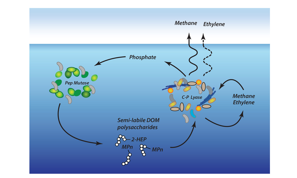
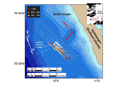
Figure 1. Ocean waters overlying shallow-water methane seeps (white dots) offshore from the Svalbard Islands absorb substantially more atmospheric carbon dioxide than the methane that they emit to the atmosphere. Colors indicate the strength of the negative greenhouse warming potential associated with carbon dioxide influx to these surface waters relative to the positive greenhouse warming potential associated with the methane emissions. Gray shiptracks have background values for the relative greenhouse warming potential.

Analysis of the data confirmed that methane was entering the atmosphere above the shallowest (water depth of 260-295 feet or 80-90 meters) Svalbard margin seeps. The data also showed that significant amounts of CO2 were being absorbed by the waters near the ocean surface, and that the cooling effect resulting from CO2 uptake is up to 230 times greater than the warming effect expected from the methane emitted.

Most previous studies have focused only on the sea-air flux of methane overlying seafloor seep sites and have not accounted for the drawdown of CO2 that could offset some of the atmospheric warming potential of the methane. Phytoplankton appeared to be more active in the near-surface waters overlying the seafloor methane seeps, which would explain why so much carbon dioxide was being absorbed. Physical and biogeochemical measurements of near-surface waters overlying the seafloor methane seeps showed strong evidence of upwelling of cold, nutrient-rich waters from depth, stimulating phytoplankton activity and increasing CO2 drawdown. This study was the first to document this CO2 drawdown mechanism in a methane source region.

“If what we observed near Svalbard occurs more broadly at similar locations around the world, it could mean that methane seeps have a net cooling effect on climate, not a warming effect as we previously thought,” said USGS biogeochemist John Pohlman, the paper’s lead author. “We are looking forward to testing the hypothesis that shallow-water methane seeps are net greenhouse gas sinks in other locations.”


Authors:
John W. Pohlman (USGS Woods Hole Coastal & Marine Science Center)
Jens Greinert (GEOMAR, Univ. of Tromsø, Royal Netherlands Institute for Sea Research)
Carolyn Ruppel (USGS Woods Hole Coastal & Marine Science Center)
Anna Silyakova (Univ. of Tromsø)
Lisa Vielstädte (GEOMAR)
Michael Casso (USGS Woods Hole Coastal & Marine Science Center)
Jürgen Mienert (Univ. of Tromsø)
Stefan Bünz (Univ. of Tromsø)

Seasonal forecasts of ocean conditions in the California Current Large Marine Ecosystem

Posted by mmaheigan 
· Thursday, February 16th, 2017 

The California Current Large Marine Ecosystem (CCLME) is a productive coastal ecosystem extending from Baja California, Mexico, to British Columbia, Canada. High primary productivity is sustained by inputs of cooler, nutrient-rich waters during seasonal wind-driven upwelling in spring and summer. This high productivity fuels higher trophic levels, including highly valued commercial ($3.5B yr-1) and recreational ($2.5B yr-1) US fisheries (NOAA 2016). The CCLME system experiences large interannual and decadal variability in ocean conditions in response to the El Niño-Southern Oscillation (ENSO) and extratropical climate modes such as the Pacific Decadal Oscillation and the North Pacific Gyre Oscillation (Di Lorenzo et al. 2013). ENSO events affect productivity of the CCLME ecosystem through atmospheric and oceanic pathways. In the former, El Niño triggers a decrease in equatorward winds (Alexander et al. 2002), reducing upwelling and nutrient inputs to coastal surface waters (Schwing et al. 2002; Jacox et al. this issue). In the latter, El Niño events propagate poleward from the equator via coastally trapped Kelvin waves, increasing the depth of the thermocline, and hence decreasing the nutrient concentration of upwelled source waters during El Niño events (Jacox et al. 2015; Jacox et al. this issue). Thus, CCLME productivity, forage fish dynamics, and habitat availability for top predators can vary substantially between years (Chavez et al. 2002; Di Lorenzo et al. 2013; Hazen et al. 2013; Lindegren et al. 2013), and there is increasing recognition of the need to incorporate seasonal forecasts of ocean conditions into management frameworks to improve fisheries management and industry decisions (Hobday et al. 2016; Tommasi et al. 2017a). We describe herein recent improvements in the seasonal prediction of ENSO and how these advances have translated to skillful forecasts of oceanic conditions in the CCLME. We conclude by offering remarks on the implications for ecological forecasting and improved management of living marine resources in the CCLME.

Seasonal ENSO predictions

ENSO is the dominant mode of seasonal climate variability, and while it is a tropical Pacific phenomenon, its effects extend over the entire Pacific basin and even globally. ENSO and its teleconnections influence rainfall, temperature, and extreme events such as flooding, droughts, and tropical cyclones (Zebiak et al. 2015). Because of the extensive societal impacts associated with ENSO, its prediction has been central to the development of today’s state-of–the-art seasonal climate prediction systems. The first attempts at ENSO prediction go back to the 1980s (Cane et al. 1986). Today, resulting from the development of an ENSO observing system located in the equatorial Pacific (McPhaden et al. 1998) and large improvements in our understanding of ENSO dynamics over the last two decades (Neelin et al. 1998; Latif et al. 1998; Chen and Cane 2008), prediction systems can, in general, skillfully predict ENSO up to about six months in advance (Tippett et al. 2012; Ludescher et al. 2014). While such skillful ENSO forecasts may also improve prediction of the extratropical ENSO response, intrinsic variability of the extratropical atmosphere and ocean, and the chaotic nature of weather, will limit extratropical prediction skill no matter how accurately the models—and observations initializing them—predict ENSO itself. ENSO operational forecasts from numerous climate modeling centers are made available in real-time from Columbia University’s International Research Institute for Climate and Society and NOAA’s Climate Prediction Center.

Given its global impact, ENSO provides much of the climate forecasting skill on seasonal timescales (Goddard et al. 2001). While weather is only predictable over a timescale of days (up to about two weeks) owing to the chaotic nature of the atmosphere (Lorenz 1963), predictions of seasonal-scale anomalies are possible because of the ability of global dynamical prediction systems to model atmosphere-ocean coupling processes and other atmosphere forcing factors, such as land and sea ice, which vary more slowly than the atmosphere (Goddard 2001). Low-frequency variations in sea surface temperature (SST), particularly in the tropics, can modulate the atmosphere (as is the case for ENSO), making some weather patterns more likely to occur over the next month or season. Therefore, the ability of the coupled global climate models to skillfully forecast the evolution of observed tropical SSTs, shifts the distribution of likely average weather over the next month or season may be, and allows for skillful prediction of seasonal climate anomalies.

While seasonal predictability is relatively high for SST due to the ocean’s large thermal inertia, assessments of SST predictability have largely been focused on ocean basin-scale modes of variability (e.g., ENSO), linked to regional rainfall and temperature patterns over land. However, recent work has demonstrated that seasonal SST predictions are also skillful in coastal ecosystems (Stock et al. 2015; Hervieux et al. 2017), and, as detailed in the next section, specifically for the CCLME (Jacox et al. 2017).

Seasonal climate predictions in the California Current Large Marine Ecosystem

Recent advances in ENSO prediction and global dynamical seasonal climate prediction systems have enabled skillful seasonal forecasts of SST anomalies in the CCLME after bias correcting the forecasts to remove model drift (Stock et al. 2015; Jacox et al. 2017; Hervieux et al. 2017). Skill of SST anomaly predictions produced by the National Oceanic and Atmospheric Administration (NOAA) North American Multi-Model Ensemble (NMME) is shown in Figure 1. Skill is evaluated through the anomaly correlation coefficient (ACC) between monthly SST anomalies from retrospective forecasts from 1982 to 2009 and observed SST anomalies. Forecasts are skillful (ACC > 0.6) across initialization months for lead times up to about four months (Figure 1). Persistence of the initialized SST anomalies provides much of the prediction skill at these short lead times (Stock et al. 2015; Jacox et al. 2017). Preexisting temperature anomalies at depth may also provide some predictability. Skillful forecasts of February, March, and April SST extend to lead times greater than six months (Figure 1; Stock et al. 2015; Jacox et al. 2017). This ridge of enhanced predictive skill in winter to early spring forecasts is apparent across seasonal forecasting models and arises from the ability of the prediction systems to capture the wintertime coastal signature of predictable basin-scale SST variations (Stock et al. 2015; Jacox et al. 2017). Specifically, the models can skillfully forecast the predictable evolution of meridional winds during ENSO events and the associated changes in upwelling anomalies and SST in the CCLME (Jacox et al. 2017).

Figure 1. Anomaly correlation coefficients (ACCs) as a function of forecast initialization month (x-axis) and lead-time (y-axis) for (left) persistence and (right) NOAA NMME mean for the California Current system (US West Coast, less than 300 km from shore). Note the ridge of high SST anomaly prediction skill exceeding persistence at long lead-times (4-12 months) for late winter-early spring forecasts. Grey dots indicate ACCs significantly above zero at a 5% level; white dots indicate ACCs significantly above persistence at a 5% level. (Adapted from Jacox et al. 2017).


Owing to the severe ecological and economic consequences of extreme SST conditions in the CCLME (e.g., Cavole et al. 2016), it is also instructive to look at forecast performance over time, specifically during the CCLME extreme warm events of 1991-1992, 1997-1998, and 2014-2016, and the CCLME extreme cold events of 1988-1989, 1998-1999, and 2010-2011 (Figure 2). All of the cold events were associated with La Niña conditions, and the first two warm events and 2015-2016 were associated with El Niño. However, the anomalously warm conditions of 2014 and 2015, dubbed “the blob,” were caused by a resilient ridge of high pressure over the North American West Coast that suppressed storm activity and mixing, and allowed a build-up of heat in the upper ocean (Bond et al. 2015).

The forecast system is highly skillful at one-month lead times. It is also skillful at longer lead times of three and six months, as seen by the forecasted February to April SSTs following the 2010-2011 La Niña and the 2015-2016 El Niño (Figure 2). However, at these longer lead times, the forecast system was unable to capture the extreme magnitude of the warm “blob” anomalies during 2014 and 2015 (Figure 2). Also, while fall to winter conditions during the 1991-1992 El Niño and the late winter-early spring conditions following the 1997-1998 El Niño were forecasted with a six-month lead time, the prolonged warm conditions over the 1992 summer and the early transition to anomalously warm conditions during the summer of 1997 were not (Figure 2).

Transitions in and out of the 1991 and 1997 El Niño events were particularly unusual also at the Equator, with El Niño conditions developing late in 1991 and persisting well into the summer of 1992, and El Niño conditions appearing early in summer 1997 (see Figure 2 in Jacox et al. 2015). The spring predictability barrier for ENSO (i.e., a dip in forecast skill for forecasts initialized over the ENSO transition period of March-May; Tippet et al. 2012), as well as weaker teleconnections to the extratropics in summer, may partly explain the lower forecast skill for these El Niño events during summer and fall, and the poorer forecast performance in predicting the early transition to La Niña conditions in 1998-1999 and 2010-2011 (Figure 2).

The forecast system was also unable to predict the cooler conditions over the ENSO-neutral spring and summer of 1991 (Figure 2). The conditional predictability of CCLME winds and SST on ENSO implies that during ENSO-neutral conditions, such as in 1991 and 2014, forecasts of winds are not skillful and SST forecast skill is therefore limited to lead times up to about four months (Jacox et al. 2017). Thus, skillfulness of the seasonal predictions results from a complex interplay of factors that will require further study to identify the underlying mechanisms driving differing levels of robustness.

Figure 2. Predictions at 1-month (red line), 3-month (blue line), and 6-month (green line) lead times of SST anomalies (°C) for the CCLME from the NOAA Geophysical Fluid Dynamics Laboratory (GFDL) CM2.5 FLOR global climate prediction systems and Reynolds OISST.v2 observations (black line) for specific extreme events in the CCLME. Warm events are on the left; cold events are on the right. The dotted lines represent the February to April period of enhanced predictive skill following ENSO events. The x-axis is months since January 1 of the year in which the extreme event started.


Seasonal forecasts for fisheries management applications

While seasonal prediction of living marine resources has been a goal for the past three decades (GLOBEC 1997), operational use of seasonal SST forecasts to inform dynamic management of living marine resources was pioneered in Australia (Hobday et al. 2011), where seasonal SST forecasts are now used to improve the decision making of the aquaculture industry (Spillman and Hobday 2014; Spillman et al. 2015), fishers (Eveson et al. 2015), and fisheries managers (Hobday et al. 2011). Through both increased awareness of climate prediction skill at fishery-relevant scales and of their value to ecosystem-based management, such efforts have now begun to expand to other regions (see Tommasi et al. 2017a, and case studies therein). In the CCLME, recent work has demonstrated that integration of current March SST forecasts into fisheries models can provide useful information for catch limit decisions for the Pacific sardine fishery (i.e., how many sardines can be caught each year?) when combined with existing harvest cutoffs (Tommasi et al., 2017b). Knowledge of future SST conditions can improve predictions of future recruitment and stock biomass and allow for the development of a dynamic management framework, which could increase allowable fisheries harvests during periods of forecasted high productivity and reduce harvests during periods of low productivity (Tommasi et al. 2017b). Hence, integration of skillful seasonal forecasts into management decision strategies may contribute to greater long-term catches than those set by management decisions based solely on either past SST information or on no environmental information at all (Figure3; Tommasi et al., 2017b).

Figure 3. Mean long-term Pacific sardine catch and biomass following catch limit decisions integrating different levels of environmental information. The catch limit incorporating future SST information reflects the uncertainty of a 2-month lead forecast. (Adapted from Tommasi et al. 2017b).


Novel dynamical downscaling experiments in the Northern California Current as part of the JISAO Seasonal Coastal Ocean Prediction of the Ecosystem (J-SCOPE) project (Siedlecki et al. 2016) show that seasonal regional climate forecasts may also be of potential utility for dynamic spatial management strategies in the CCLME (Kaplan et al. 2016). Predictions of ocean conditions from a global dynamical climate prediction system (NOAA NCEP CFS) forced the Regional Ocean Modeling System (ROMS) with biogeochemistry to produce seasonal forecasts of ocean conditions, both at the surface and at depth, with measureable skill up to a four-month lead time (Siedlecki et al. 2016). The downscaling both enables forecasts of fishery-relevant biogeochemical variables such as chlorophyll, oxygen, and pH not yet produced by global forecasting systems, and resolves the fine-scale physical and ecological processes influencing the distribution of managed species within the CCLME. For instance, high-resolution regional implementations of ROMS resolve upwelling and coastal wave dynamics (Jacox et al. 2015; Siedlecki et al. 2016), two processes that drive the CCLME response to ENSO variability, better than coarser-resolution global models. Downscaled forecasts have also driven prototype forecasts of Pacific sardine spatial distribution (Kaplan et al. 2016). Such forecasts have the potential to inform fishing operations, fisheries surveys, and US and Canadian quotas for this internationally shared stock (Kaplan et al. 2016; Siedlecki et al. 2016; Tommasi et al. 2017a).

These CCLME case studies suggest that with recent advancements in state-of-the-art global dynamical prediction systems and regional downscaling models, some skillful seasonal predictions of ocean conditions are possible (Siedlecki et al. 2016; Tommasi et al. 2017a). Seasonal forecast skill may be further improved by improved representation of other features such as ocean eddies and gyre circulations in the extratropics and the basin-wide atmospheric response to SST anomalies in the Kuroshio-Oyashio region (Smirnov et al. 2015). Such skillful seasonal forecasts present opportunities for inclusion in adaptive management strategies for improved living marine resource management and better informed industry operations in the CCLME.


Authors

Desiree Tommasi (Princeton University)
Michael G. Jacox (University of California, Santa Cruz, NOAA Southwest Fisheries Science Center)
Michael A. Alexander Earth System Research Laboratory, NOAA
Francisco E. Werner (NOAA Southwest Fisheries Science Center)
Samantha Siedlecki (University of Washington)
Charles A. Stock Geophysical Fluid Dynamics Laboratory, NOAA
Nicholas A. Bond (University of Washington)

References

Alexander, M. A., I. Bladé, M. Newman, J. R. Lanzante, N. C. Lau, and J. D. Scott, 2002: The atmospheric bridge: The influence of ENSO teleconnections on air-sea interaction over the global oceans. J. Climate, 15, 2205-2231, doi: 10.1175/1520-0442(2002)015<2205:TABTIO>2.0.CO;2.

Bond, N. A., M. F. Cronin, H. Freeland, and N. Mantua, 2015: Causes and impacts of the 2014 warm anomaly in the NE Pacific. Geophys. Res. Lett., 42, 3414–3420, doi:10.1002/2015GL063306.

Cane, M. A., S. E. Zebiak, and S. C. Dolan, 1986: Experimental forecasts of El Niño. Nature 321, 827–832, doi:10.1038/321827a0.

Cavole, L. M., and Coauthors, 2016: Biological impacts of the 2013–2015 warm-water anomaly in the Northeast Pacific: Winners, losers, and the future. Oceanogr., 29, 273–285, doi: 10.5670/oceanog.2016.32.

Chavez, F. P., J. T. Pennington, C. G. Castro, J. P. Ryan, R. P. Michisaki, B. Schlining, P. Walz, K. R. Buck, A. McFadyen, and C. A. Collins, 2002: Biological and chemical consequences of the 1997–1998 El Niño in central California waters. Prog. Oceanogr., 54, 205–232, doi: 10.1016/S0079-6611(02)00050-2.

Chen, D., and M. A. Cane, 2008: El Niño prediction and predictability. J. Comp. Phys., 227, 3625-3640, doi: 10.1016/j.jcp.2007.05.014.

Di Lorenzo, E., and Coauthors, 2013: Synthesis of Pacific Ocean climate and ecosystem dynamics. Oceanogr. 26, 68–81, doi: 10.5670/oceanog.2013.76.

Eveson, J. P., A. J. Hobday, J. R. Hartog, C. M. Spillman, and K. M. Rough, 2015: Seasonal forecasting of tuna habitat in the Great Australian Bight. Fish. Res., 170, 39–49 doi: 10.1016/j.fishres.2015.05.008.

Global Ocean Ecosystem Dynamics (GLOBEC), 1997: Global Ocean Ecosystem Dynamics Science Plan. R. Harris and the members of the GLOBEC Scientific Steering Committee, Eds., IGBP secretariat, Stockholm, Sweden, 83 pp.

Goddard, L., S. J. Mason, S. E. Zebiak, C. F. Ropelewski, R. Basher, and M. A. Cane, 2001: Current approaches to seasonal-to-interannual climate predictions. Int. J. Climatology, 21, 1111–1152, doi: 10.1002/joc.636.

Hazen, E. L., and Coauthors, 2013: Predicted habitat shifts of Pacific top predators in a changing climate. Nat. Climate Change, 3, 234-238, doi:10.1038/nclimate1686.

Hervieux, G., M. Alexander, C. Stock, M. Jacox, K. Pegion, and D. Tommasi, 2017: Seasonal sea surface temperature anomaly prediction skill for coastal ecosystems using the North American multi-model ensemble (NMME). Climate Dyn., submitted.

Hobday, A. J., J. R. Hartog, C. M. Spillman, and O. Alves, 2011: Seasonal forecasting of tuna habitat for dynamic spatial management. Can. J. Fish. Aq. Sci., 68, 898-911, doi: 10.1139/f2011-031.

Hobday, A. J., C. M. Spillman, J. P. Eveson, and J. R. Hartog, 2016: Seasonal forecasting for decision support in marine fisheries and aquaculture. Fish.,. Oceanogr., 25, 45-56, doi: 10.1111/fog.12083.

Jacox, M. G., J. Fiechter, A. M. Moore, and C. A. Edwards, 2015: ENSO and the California Current coastal upwelling response. J. Geophys. Res. Oceans, 120, 1691–1702, doi:10.1002/ 2014JC010650.

Jacox, M., E. L. Hazen, K. D. Zaba, D. L. Rudnick, C. A. Edwards, A. M. Moore, and S. J. Bograd, 2016: Impacts of the 2015–2016 El Niño on the California Current System: Early assessment and comparison to past events. Geophys. Res. Lett. 43, 7072-7080, doi:10.1002/2016GL069716.

Jacox, M. G., M. A. Alexander, C. A. Stock, and G. Hervieux, 2017: On the skill of seasonal sea surface temperature forecasts in the California Current System and its connection to ENSO variability. Climate Dyn., in review.

Kaplan, I. C., G. D. Williams, N. A. Bond, A. J. Hermann, and S. Siedlecki, 2016: Cloudy with a chance of sardines: forecasting sardine distributions using regional climate models. Fish. Oceanogr., 25, 15–27, doi: 10.1111/fog.12131.

Latif, M., A. Sterl, E. Maier-Reimer, and M. M. Junge, 1998: Climate variability in a coupled GCM. Part I: the tropical Pacific. J. Climate, 6, 5–21, doi: 10.1175/1520-0442(1993)006<0005:CVIACG>2.0.CO;2.

Lindegren, M., D. M. Checkley Jr., T. Rouyer, A. D. MacCall, and N. C. Stenseth, 2013: Climate, fishing, and fluctuations of sardine and anchovy in the California Current. Proc. Nat. Acad. Sci., 110, 13672-13677, doi: 10.1073/pnas.1305733110.

Lorenz, E. N. 1963: Deterministic nonperiodic flow. J. Atmos. Sci., 20, 130-141, doi: 10.1175/1520-0469(1963)020<0130:DNF>2.0.CO;2.

Ludescher, J., A. Gozolchiani, M. Bogachev, A. Bunde, S. Havlin, and H. J. Schellnhuber, 2014: Very early warning of next El Niño. Proc. Nat. Acad. Sci., 111, 2064-2066, doi: 10.1073/pnas.1323058111.

McPhaden, M. J., and Coauthors, 1998: The TOGA observing system: a decade of progress. J. Geophys. Res., 103, 14,169-14,240, doi: 10.1029/97JC02906.

Neelin, J. D., D. S. Battisti, A. C. Hirst, F. F. Jin, Y. Wakata, T. Yamagata, and S. E. Zebiak, 1998: ENSO theory. J. Geophys. Res., 103, 14261–14290, doi: 10.1029/97JC03424.

NOAA, 2016: National Marine Fisheries Service Seafood Industry Impacts tool. https://www.st.nmfs.noaa.gov/apex/f?p=160:1.

Schwing, F. B., T. Murphree, L. DeWitt, and P. M. Green, 2002: The evolution of oceanic and atmospheric anomalies in the northeast Pacific during the El Niño and La Niña events of 1995–2001. Prog. Oceanogr., 54, 459–491, doi:10.1016/S0079-6611(02)00064-2.

Siedlecki, S. A., I. C. Kaplan, A. J. Hermann, T. T. Nguyen, N. A. Bond, J. A. Newton, G. D. Williams, W. T. Peterson, S. R. Alin, and R. A. Feely, 2016: Experiments with seasonal forecasts of ocean conditions for the northern region of the California Current upwelling system. Sci. Rep., 6, 27203, doi: 10.1038/srep27203.

Smirnov, D., M. Newman, M. A. Alexander, Y.-O. Kwon, and C. Frankignoul, 2015: Investigating the local atmospheric response to a realistic shift in the Oyashio sea surface temperature front. J. Climate, 28, 1126-1147, doi: 10.1175/JCLI-D-14-00285.1.

Spillman, C. M., J. R. Hartog, A. J. Hobday, and D. Hudson, 2015: Predicting environmental drivers for prawn aquaculture production to aid improved farm management. Aquaculture, 447, 56–65, doi: 10.1016/j.aquaculture.2015.02.008.

Spillman, C. M., and A. J. Hobday, 2014: Dynamical seasonal ocean forecasts to aid salmon farm management in a climate hotspot. Climate Risk Management, 1, 25-38, doi: 10.1016/j.crm.2013.12.001.

Stock, C. A., K. Pegion, G. A. Vecchi, M. A. Alexander, D. Tommasi, N. A. Bond, P. S. Fratantoni, R. G. Gudgel, T. Kristiansen, T. D. O’Brien, Y. Xue, and X. Yang, 2015: Seasonal sea surface temperature anomaly prediction for coastal ecosystems. Prog. Oceanogr., 137, 219-236, doi: 10.1016/j.pocean.2015.06.007.

Tippett, M. K., A. G. Barnston, and S. Li, 2012: Performance of recent multi-model ENSO forecasts. J. App. Meteorol. Climatol., 51, 637–654, doi: 10.1175/JAMC-D-11-093.1.

Tommasi, D., and Coauthors, 2017a. Managing living marine resources in a dynamic environment: the role of seasonal to decadal climate forecasts. Prog. Oceanogr., doi: 10.1016/j.pocean.2016.12.011.

Tommasi, D., C. Stock, K. Pegion, G. A. Vecchi, R. D. Methot, M. Alexander, and D. Checkley, 2017b: Improved management of small pelagic fisheries through seasonal climate prediction. Ecol. App., doi: 10.1002/eap.1458.

Zebiak, S. E., B. Orlove, A. G. Muñoz, C. Vaughan, J. Hansen, T. Troy, M. C. Thomson, A. Lustig, and S. Garvin, 2015: Investigating El Niño-Southern Oscillation and society relationships. WIREs Climate Change, 6, 17–34, doi: 10.1002/wcc.294.


A New Explanation for the Marine Methane Paradox

Posted by mmaheigan 
· Thursday, February 2nd, 2017 

A large fraction of the ocean-to-atmosphere flux of methane occurs in well-oxygenated, open ocean oligotrophic gyres, a phenomenon seemingly at odds with well-known pathways of archaeal methane production under strictly anaerobic conditions. Nearly a decade ago, David Karl and colleagues at the University of Hawaii proposed that water column methane could arise from bacterial metabolism of methylphosphonate, a simple organic compound with reduced phosphorus bonded directly to carbon. However, evidence for this pathway in the environment was lacking. In a recent study published in Nature Geoscience, Repeta et al. (2016) were able to test Karl’s hypothesis using a combination of microbial incubations, genomic analyses, and in-depth chemical analyses of marine dissolved organic matter (DOM). The study revealed that polysaccharides decorated with methyl- and hydroxyethylphosphonate esters are abundant throughout the water column, and that methane and ethylene were quickly produced by natural consortia of bacteria exposed to DOM-amended seawater. Companion knock-out experiments of bacteria isolates further showed that the C-P lyase metabolic pathway was responsible for methane production. Daily cycling of only 0.25% DOM polysaccharide can easily support measured fluxes of marine methane to the atmosphere. Figure from Repeta et al. (2016).

What controls the distribution of dissolved organic carbon in the surface ocean?

Posted by mmaheigan 
· Friday, November 11th, 2016 

Around 662 billion tons of organic carbon are dissolved in the ocean, making the pool one of Earth’s major, exchangeable carbon reservoirs. Dissolved organic carbon (DOC) has many ecological functions. It can form complexes with metals (1); absorb UV and visible light, acting as a “sunscreen” for marine microorganisms and controlling primary production in the upper water column (2); it has antioxidant activity, reacting with free radicals in the media (3); but most importantly, it serves as substrate for the microbial loop and as a vehicle for carbon sequestration in the ocean. Therefore, DOC plays an important role in climate on geological time scales.

Because the amount of atmospheric CO2 is of the same magnitude as the DOC pool, and is closely linked to it through exchange, variations in one of these reservoirs can affect the other, impacting the carbon cycle with consequences for climate. Significant net DOC remineralization would lead to an increase of atmospheric CO2, enhancing greenhouse warming at the surface of the Earth. Net oxidation of only 1% of the seawater DOC pool within 1 year would be sufficient to generate a CO2 flux of 7 PgC/yr, comparable to that produced annually by fossil fuel combustion (4). It has also been proposed that a large-scale oxidation of DOC may have prevented a dramatic global glaciation (‘snowball earth’) in the Neoproterozoic period (5).

Despite its importance, knowledge about DOC dynamics is relatively limited; in fact, it was considered highly inert until about three decades ago when a new analytical technique for measuring it via high-temperature catalytic oxidation stimulated new interest (6). The technique eventually provided more accurate DOC values, showing that it was more involved in the carbon cycle than previously thought and that its concentrations vary with depth, time, and location. Considering DOC distributions observed in the surface Atlantic Ocean (Fig. 1), we see values in the subtropical gyres of 65-70 µmol Kg-1, the highest concentrations in the tropics (> 70 µmol Kg-1), the lowest in the Southern Ocean (< 50 µmol Kg-1), and moderate concentrations in the northern North Atlantic (55-60 µmol Kg-1); this pattern is consistent in other ocean basins. So what controls this distribution and can we predict it? Even with improved analytical techniques, DOC is not a variable that can be measured easily at sea, and the sampling must be done carefully since it is easy to contaminate. Therefore, DOC data are typically fewer than those of other more readily determined variables such as nutrients and oxygen. If we could predict DOC from variables for which much greater global ocean coverage exists, we could fill the very large spatial and temporal gaps in the DOC fields.

DOC is produced in the upper water column by phytoplankton (primary producers). Actually, half of the inorganic carbon that is fixed by phytoplankton is transformed to DOC. Heterotrophic microbes consume most of that DOC, but ~ 4% of global annual net primary production (~ 2 Pg C y-1) (7) accumulates as DOC, much of which is exported to the mesopelagic via vertical mixing and convergence, thus contributing to the biological carbon pump.

New primary production, the foundation of a system’s net community production (NCP), depends on new nutrients reaching the euphotic zone, which happens primarily via upwelling in divergence zones and winter vertical mixing. NCP is the balance of the carbon generated by primary producers minus that lost through heterotrophic respiration (prokaryotes and animals). It can be estimated either by a loss of reactants (CO2 or nutrients) or a gain in products (suspended POC, DOC, and export production) (8).

In our work, we needed to establish the fraction of NCP that was present in dissolved form (i.e., the net DOC production ratio, or NDPr). For that, we simply estimated NCP from the nitrate (NO3–) that is consumed in the euphotic zone (DNO3–):

ΔNO3– = new NO3– (introduced from deeper layers) – remaining NO3– (at surface) (Eq. 1)

In the same way, we also calculated net accumulated DOC, or ΔDOC:

ΔDOC = DOC in euphotic zone – DOC introduced from deeper layers (Eq. 2)

The ratio between ΔDOC and ΔNO3– gave us the NDPr:

NDPr = ΔDOC/ΔNO3– (Eq. 3)

NDPr was calculated throughout the Atlantic Ocean using observations of DOC and NO3– from >15 international oceanographic cruises over the last decade, including those occupied by the US Repeat Hydrography program (Fig. 1). Values of NDPr mostly varied between 0.1 and 0.4 (Fig. 2), with the exception of the North Atlantic Subtropical Gyre (NASG), where NDPr values reach >0.8 at times. After sensitivity testing, we applied a NDPr value of 0.17 to the entire basin, which yielded the smallest error between calculated and observed DOC concentrations. Applying this NDPr value to ΔNO3– (i.e. NCP) obtained from cruise data, we estimate ΔDOC (Eq. 4), in which 6.6 is the molar conversion from N to C units:

ΔDOC= ΔNO3– * 6.6 * 0.17 = NCP * 0.17 (Eq. 4)

To obtain the calculated DOC concentration (DOCcalculated), we added the DOC concentration of underlying source waters (DOCsource) to ΔDOC (Eq. 5):

DOCcalculated = DOCsource + ΔDOC (Eq. 5)

When comparing calculated vs. observed DOC (Fig. 3), we found significant agreement (R2 = 0.64; p < 0.001; n=268) throughout the Atlantic, except in the western North Atlantic, where observed DOC > estimated DOC, especially in the southern sector. After this validation of our approach using nutrients and DOC observations, we applied the method to the more extensive NO3– distributions available in the World Atlas Ocean (WOA) climatology to develop a DOCcalculated map for the entire Atlantic (Fig. 4a). The calculated values agree well with the observations, with a total error of 8.94%.

How much DOC is annually produced in the surface Atlantic Ocean? Total organic carbon export (considered equivalent to NCP) in the Atlantic has been estimated to be 4.15-4.3 Pg C y-1 (9, 10). Applying the 0.17 NDPr (equation 3) indicates that 0.70-0.75 Pg C y-1 accumulates in the Atlantic surface as DOC; as such, the Atlantic accounts for ~36% of the global net DOC production ~2 Pg C y-1.

In permanently stratified areas like the southern sectors of the NASG, our approach is invalid since there is little nutrient input from underlying depths. Also, the static view of our approach does not take into account advection that will modify the DOC distributions, nor does it account for eventual removal of accumulated and advected DOC by microbes. To account for these influences on distributions, we applied the ΔNO3– measurements to a steady-state ocean circulation model including terrestrial DOC inputs and DOC remineralization (Fig. 4b). In the model, zonal advection is evident through enrichment of DOC in the Caribbean Sea. Also, inputs of terrestrial DOC are observed near the outflow of the Amazon River. However, the model only slightly improved the match between observations and modeled DOC, with a total error of 8.71% vs. the 8.94% obtained before the model application.

The correspondence between observations and modeled values was good, considering that we are comparing observations of DOC from cruises during specific seasons with estimates based on more idealized nutrient climatology. The main mismatch is found in the western NASG, where observations can reach 13 µmol Kg-1 higher than calculated values. Local production and/or allochthonous inputs of either new nutrients or DOC must be considered. Local production of DOC could result from addition of nitrogen from sources beyond vertical mixing such as diazotrophic N2 fixation, atmospheric deposition, and river runoff. Alternatively, DOC can be concentrated by evaporation, as is sea salt. However, none of these explain the high DOC values observed in the NASG. DOC flux estimated from dissolved organic nitrogen (DON) released by N2 fixation (11) is too low to explain the extra DOC. Regarding the atmospheric deposition, aerosol optical depth data suggest higher deposition in the eastern than in the western North Atlantic (11), and no excess of DOC is observed there. According to salinity distributions from the World Ocean Atlas, advection of DOC from the closest major rivers (Amazon and Orinoco) does not extend far enough northward to explain the NASG anomaly. Salinity normalization of DOC does not erase the feature, indicating that evaporation is not the cause. Those elevated values of carbon are found during cruises from 2003 in the same area (12), so it appears to be a persistent feature. The anomaly also coincides with a DON maximum and a light stable isotope (δ15N) composition in the particulate organic carbon based on measurements recorded in 2004 (13). An explanation for these anomalies has not been confirmed.


Conclusions

New nutrients are the fundamental driver of net DOC accumulation in the surface Atlantic Ocean. As such, climate-driven changes in ocean dynamics, which will affect the supply of nutrients to the euphotic zone, will affect the DOC inventory. The effects of climate change on the nutrient supply to the upper water column are not well known, but they will depend on the opposing influences of thermal stratification and upwelling intensification. Some authors predict an intensification and spatial homogenization of coastal upwelling systems (14, 15). Such would increase the nutrient input to the euphotic zone and the net DOC production. In contrast, others have reported that ocean warming should intensify thermal stratification, reducing nutrient flux by vertical mixing in regions not affected by coastal upwelling systems (16, 17). Depending on which of these phenomena dominate, the nutrient supply will change, in turn changing the DOC budget and its distribution. Furthermore, the percentage of NCP accumulating as DOC (i.e. NDPr), found here to be ~17%, could change in response to a shift in the balance of autotrophs and heterotrophs. This multitude of influencing factors will undoubtedly impact the future course of the oceanic DOC budget.


Authors

Cristina Romera-Castillo (Univ. of Vienna) and Dennis A. Hansell (RSMAS, Univ. Miami)

Acknowledgments

The authors thank the other co-author, Robert T. Letscher, from the more extended version of this published work. Also to Dr. X.A. Álvarez-Salgado for the use of DOC data he collected during cruises supported by the Spanish government. Data collection on US CLIVAR sections and involvement by C.R.-C. and D.A.H. were supported by US National Science Foundation OCE1436748.

References

  1. Midorikawa, T., E. Tanoue, 1998. Mar. Chem. 62, 219-239.
  2. Arrigo, K. R., C. W., Brown, 1996. Mar. Ecol. Prog. Ser. 140, 207-216.
  3. Romera-Castillo, C., R. Jaffé, 2015. Mar. Chem. 177, 668–676.
  4. Hedges, J. I. 2002. In: Hansell, D., Carlson, C. (Eds.), 2002. Biogeochemistry of marine dissolved organic matter. Academic Press, San Diego, pp. 1-33.
  5. Peltier, W. R. et al., 2007. Nature 450, 813-819.
  6. Hansell, D. A., C. A. Carlson, 2015. Eos, 96, doi:10.1029/2015EO033011.
  7. Hansell, D. A., et al., 2009. Oceanography 22, 202-211.
  8. Hansell, D. A., C. A. Carlson, 1998. Global Biogeochem. Cycles 12, 443-453.
  9. Laws, E. A., et al., 2000. Global Biogeochem. Cycles 14, 1231-1246.
  10. Dunne, J. P., et al., 2007. Global Biogeochem. Cycles 21, GB4006.
  11. Benavides, M., et al., 2013. J. Geophys. Res.: Oceans 118, 3406-3415.
  12. Carlson, C. A. et al., 2010. Deep-Sea Res. Pt II 57, 1433-1445.
  13. Landolfi, A. et al., 2016. Deep-Sea Res. Part I 111, 50-60.
  14. Sydeman, W. J. et al., 2014. Science 345, 77-80.
  15. Wang, D. et al., 2015. Nature 518, 390-394.
  16. Cermeño, P. et al., 2008. PNAS 105, 20344-20349.
  17. Bopp L, et al., 2013. Biogeosciences 10, 6225-6245.
  18. Schlitzer, R., 2015. Ocean Data View. Available at https://odv.awi.de
  19. Romera-Castillo, C. et al., 2016. PNAS 113, 10497–10502.

Trace metal uptake and remineralization and their impact on upper ocean stoichiometry

Posted by mmaheigan 
· Wednesday, July 6th, 2016 

1. Stoichiometry of metals in the ocean

The close relationship between the stoichiometry of nutrients dissolved in the upper ocean and the planktonic organisms that grow in these waters has long been recognized (1, 2). The stoichiometry of 106 C:16 N:1 P first summarized by Redfield has become a fundamental concept of marine biogeochemistry, with numerous studies using the ratio as a benchmark to assess ecosystem function. Decades after the work of Redfield, with the implementation of trace metal-clean techniques, oceanographers produced the first meaningful measurements of dissolved trace metals in the open ocean (3-5), and they found that many of the bioactive metals such as Fe, Zn, Ni, Cu and Cd are also depleted in surface waters and enriched at depth, similar to the macronutrients. Such nutrient-like behavior supported not only a growing understanding of the physiological roles that these metals play in phytoplankton physiology (6), but it also indicated that biological uptake and sub-surface remineralization were important processes for controlling the distributions of these bioactive metals in the ocean. Thus, the biogeochemical behavior of the micronutrient metals is in many ways analogous to that of the macronutrients N, P and Si.

In the open ocean far from coastal and shelf influences, dissolved concentrations of bioactive metals increase with depth at relatively consistent ratios to macronutrients (5), and these metal:nutrient remineralization ratios have been used to approximate the composition of sinking biogenic material and euphotic zone phytoplankton (7, 8). These ‘extended Redfield ratios’ have been compared to average compositions of marine phytoplankton species grown in culture (9-12),  and the general agreement between these approaches further supports the importance of biological uptake and subsequent remineralization of trace metals in the upper ocean as key processes impacting trace metal geochemistry. Average metal:nutrient stoichiometries for phytoplankton have also been compared to dissolved stoichiometries in the ambient water, and relationships between these fractions have been used to estimate nutrient limitation and deficiency in the ocean (13). Thus, there is significant interest in controls on upper ocean metal stoichiometries, as well as the relationships between cellular/biological, particulate and dissolved fractions.

Analogous to macronutrients, there are also relationships between metal stoichiometries in phytoplankton and those in deeper waters of the ocean. Departures from these relationships are likely to provide insights into the internal biogeochemical cycling of metals in the ocean. Morel and Hudson (7) noted differences in the extended stoichiometries of plankton and the water column and concluded that they must reflect the relative efficiency of remineralization of the elements, as well as the propensity of elements to be scavenged onto sinking particles in the sub-surface ocean. Similarly, the rapid remineralization of trace metals from sinking plankton was addressed in seminal work by Collier and Edmond (14). Using carefully collected data on surface plankton material, and with more computational rigor than (7), they compared surface particle stoichiometries to deep water dissolved stoichiometries and calculated the relative remineralization of plankton-associated elements in sinking biogenic material. They noted significant differences among the behaviors of biogenic metals such as Cd, Ni and Fe due to their scavenging and remineralization behaviors. More recently, Morel (15) mused about these processes and their relationships to cellular biochemistry and evolution of phytoplankton physiology and ocean biogeochemistry.

Through the GEOTRACES program, the data to test and extend these early, relatively simple box models and stoichiometric comparisons are now available. Metal concentrations and stoichiometries for phytoplankton, bulk and size-fractionated particulate material, and co-located dissolved species have been measured in the North Atlantic and South Pacific Oceans thus far. Combined with data for non-bioactive metals such as Ti and Th, these data also provide the opportunity to discern the behavior and contributions of lithogenic vs. biogenic matter, as well as the processes of remineralization and scavenging.

2. Processes affecting dissolved and particulate stoichiometries of trace metals

Vertical profiles of dissolved macronutrients show characteristic depletion at the surface and enrichment at depth due to remineralization, and dissolved micronutrients often show the same behavior. However, the internal cycling of metals in the ocean is expected to differ from that of macronutrients for a few salient reasons. Some metals such as Fe are significantly less soluble than macronutrients and are prone to abiotic adsorption onto particulate surfaces (16). This process is driven by thermodynamics, and the accompanying process of desorption also occurs; the net observed process is typically called ‘scavenging’ (Fig. 1). Scavenging in the deep ocean causes concentrations of less soluble metals such as Fe and Al to decrease along the path of thermohaline circulation, in contrast to macronutrients and more soluble metals that may mimic macronutrient behavior such as Cd and Zn (17). In the absence of significant lateral nutrient inputs, the balance of scavenging and remineralization will influence the resulting vertical profiles of dissolved elements (18).

Another key difference between macronutrients and metals is the importance of abiotic particulate fractions such as lithogenic (e.g., aeolian dust and sediment) and authigenic (e.g., Fe- and Mn-oxyhydroxide) phases. While biogenic phases are almost universally produced at the surface and remineralized with depth, abiotic phases can exhibit very different and dynamic internal cycles (19). Dust events, lateral transport and poorly constrained scavenging processes can both deliver and remove specific metals alongside biological processes. Lithogenic phases are generally denser and more refractory than biogenic particles and detritus and are thought to sink more rapidly and remineralize more slowly and at greater depth (Fig. 1; 20). Lithogenic particles may also (re)scavenge metals differently than biogenic material. Efforts to examine these processes in sinking material have been extremely limited to date, with only a few studies examining metals in trace metal-clean sediment traps (21, 22). However, recently published datasets from the GEOTRACES program are shedding new light on the multiple facets of metal partitioning and how they affect subsurface remineralization and scavenging.

A comparison of metal:phosphorus ratios in the upper ocean illuminates some of these processes. Figure 2 displays Cd:P, Fe:P, Co:P and Ni:P ratios in particles in the upper 100m, 100-300m, and 300-1,000m of the water column in the middle of the North Atlantic basin. Particulate material is sub-divided into ratios for phytoplankton cells and non-lithogenic particles (corrected for lithogenic minerals using Ti; 19). Also plotted are dissolved remineralization ratios (that is, the slope of a linear regression between the dissolved metal and phosphate) for these upper ocean depth ranges. The close coupling of Cd and P biogeochemistry has long been recognized (4), and indeed we observe very close agreement (within a factor of about 2) between dissolved Cd:P remineralization and Cd:P in surface ocean particles, as well subsurface particles. Clearly these elements are remineralizing from sinking particles at similar rates. Such comparisons of particulate and dissolved constituents need to carefully consider the different residence times of these fractions and the likelihood for lateral inputs. Here, we have chosen to focus on stations from the mid-North Atlantic gyre, where the upper 700m of the water column consists primarily of a single water mass (23).

In contrast, the remineralization of Fe and P are quickly decoupled in the water column (Fig. 2). Between 100 and 300m, typically the depth of most rapid regeneration of sinking organic material, labile particulate Fe:P has more than doubled from that in surface waters, and the Fe:P ratio of remineralized dissolved elements (0.98 mmol/mol) is more than 10-fold below that of the labile material that is sinking into these waters. Looking deeper into the water column, Fe and P continue to decouple in labile (i.e., non-lithogenic) particulates, with Fe:P of 300-1,000m particles increasing 10-fold and the dissolved remineralization ratio being nearly 1,000-fold lower (0.35 mmol/mol). Additionally, organic ligands play an important role in stabilizing dissolved Fe (24), so dissolved Fe and P ratios may be further decoupled by biological processes impacting the production and fate of these ligands (20).

A strength of GEOTRACES datasets is their wide coverage of the periodic table, and additional insights can be gained from looking at the behaviors of other bioactive trace metals that are also incorporated into sinking biogenic material. Co:P ratios in particles and remineralized dissolved fractions in the water column follow the same trend as Fe, but the decoupling of Co and P is much more subtle than with Fe, presumably due to differences in ligand coordination and Co co-oxidation with Mn (25, 26). Dissolved Co:P remineralization ratios at 100-300m generally match those found in phytoplankton and drop only 3-fold below 300m. Similarly, labile particulate Co:P ratios don’t change between 0-100m and 100-300m, also indicating that Co and P remineralize in tandem in the upper 300m. Below 300m, labile particulate Co:P increases approximately 3-fold (in contrast with Fe:P, which increases 12-fold), and this depth effect matches the effect in dissolved remineralization ratios. Thus, even though Fe and Co are considered hybrid metals that display both biological uptake and scavenging, there are clear differences in the behaviors of these metals. Nickel provides yet another perspective on the coupling of metals and P. Dissolved remineralization ratios in both subsurface depth ranges closely resemble surface ocean labile particles, supporting the biological coupling of Ni and P (5). However, residual labile particulate Ni:P increases 2- to 4-fold in successive depth ranges, indicating that remineralization is rather decoupled. Given that Ni seems to be associated with both organic material and opal frustules in diatoms (27), it may be that Ni and P are remineralized from particulate organic matter in tandem, but some Ni remains associated with sinking biogenic silica in the ocean.

3. Additional tools to explore and differentiate remineralization processes

The GEOTRACES program has welcomed the application of new analytical approaches that further enable us to study the cycling of metals in the ocean. Spectroscopy and quantitative imaging methods using synchrotron radiation have become more common in the past decade (28), and these allow us to analytically distinguish the behaviors of different fractions of particle assemblages. During the FeCycle II project, a GEOTRACES process study, the fate of Fe was tracked during a spring diatom bloom (29). Diatom cells from the dominant bloom species (Asterionellopsis glacialis) were collected in surface waters and from trace-metal clean sediment traps at 100m and 200m in the 48h following the decline of the bloom. Synchrotron x-ray fluorescence (SXRF) analyses of individual cells showed that constituent elements were lost from sinking cells at notably different rates (Fig. 3). Phosphorus was rapidly released from sinking cells, with mean P quotas decreasing 55% and 73% from surface values by 100m and 200m, respectively (30). However, only 25% of cellular Fe was lost from cells sinking through the upper 200m, while 61% of cellular Ni was remineralized. This supports the story told by the bulk biogeochemical data from the North Atlantic: Ni is remineralized largely to a similar degree as P, while Fe is lost more slowly from sinking biogenic material.

Application of microanalytical techniques such as SXRF can be combined with bulk approaches to further advance understanding of subsurface metal remineralization and cycling. In FeCycle II, Fe:P of sinking A. glacialis cells increased, on average, only 2.3-fold in the upper 200m, while Fe:P in bulk particulate matter increased more than 13-fold (30). This indicates that the behavior of sinking cells was not representative of the full particle assemblage. Iron and P were likely more completely decoupled in sinking fecal pellets and detrital material (which appears to have contributed significantly to the particulate Fe pool during FeCycle II; 31) than in intact sinking cells. Further application of this approach will allow us to not only distinguish between the behavior of biogenic and lithogenic fractions (Fig. 1), but potentially also between detrital particles. By considering metals such as Mn that are prone to oxidation and scavenging in the subsurface ocean (32, 33), it may also be possible to separate abiotic scavenging from net biological remineralization (Fig. 1). Additionally, 2D (and potentially 3D) mapping of elements within cells and particles also provides information about the spatial and potentially chemical associations of elements with particles (30, 34).

The GEOTRACES program is generating unprecedented data, both in terms of quality and quantity, regarding the cycling of bioactive trace metals in the ocean. Syntheses of these data, and integration of insights from novel microanalytical tools, as well as transcriptomic and proteomic approaches, are resulting in substantial advances in our understanding of metal biogeochemistry. No longer are we limited to a few painstakingly collected dissolved metal profiles. There is now painstakingly collected full-depth coverage of most ocean basins, including in many cases dissolved and particulate fractions of nearly all biogenic elements, enabling testing of early hypotheses about trace metal cycling and parameterization of these processes into next-generation ocean biogeochemical models.

Authors

Benjamin S. Twining, Daniel C. Ohnemus, Renee L. Torrie (Bigelow Laboratory for Ocean Sciences)

Acknowledgments

This work was funded by NSF grant OCE-1232814 to BST. RLT was funded by NSF REU grant 1460861 to Bigelow Laboratory for Ocean Sciences.

References

1. A. C. Redfield, in James Johnstone Memorial Volume, R. J. Daniel, Ed. (Liverpool University Press, 1934), pp. 176-192.
2. A. C. Redfield, Amer. Scientist 46, 205-221 (1958).
3. E. A. Boyle, J. M. Edmond, Nature 253, 107-109 (1975).
4. E. A. Boyle, F. Sclater, J. M. Edmond, Nature 263, 42-44 (1976).
5. K. W. Bruland, Earth Plan. Sci. Lett. 47, 176-198 (1980).
6. J. R. R. Frausto da Silva, R. J. P. Williams, The Biological Chemistry of the Elements: the inorganic chemistry of life. (Oxford University Press, Oxford, ed. 2nd, 2001), pp. 575.
7. F. M. M. Morel, R. J. M. Hudson, in Chemical Processes in Lakes, W. Stumm, Ed. (John Wiley & Sons, New York, 1985), pp. 251-281.
8. K. W. Bruland, J. R. Donat, D. A. Hutchins, Limnol. Oceanogr. 36, 1555-1577 (1991).
9. T. Y. Ho et al., J. Phycol. 39, 1145-1159 (2003).
10. W. G. Sunda, Marine Chem. 57, 169-172 (1997).
11. W. G. Sunda, S. A. Huntsman, Limnol. Oceanogr. 40, 132-137 (1995).
12. W. G. Sunda, S. A. Huntsman, Limnol. Oceanogr. 40, 1404-1417 (1995).
13. C. M. Moore et al., Nature Geosci. 6, 701-710 (2013).
14. R. Collier, J. Edmond, Prog. Oceanogr. 13, 113-199 (1984).
15. F. M. M. Morel, Geobiol. 6, 318-324 (2008).
16. M. Whitfield, D. R. Turner, in Aquatic Surface Chemistry: Chemical Processes at the Particle-Water Interface, W. Stumm, Ed. (John Wiley & Sons, Inc., 1987), pp. 457-493.
17. K. W. Bruland, M. C. Lohan, in The Oceans and Marine Geochemistry: Treatise on Geochemistry, H. Elderfield, Ed. (Elsevier, Oxford, 2003), pp. 23-47.
18. P. W. Boyd, M. J. Ellwood, Nature Geosci. 3, 675-682 (2010).
19. D. C. Ohnemus, P. J. Lam, Cycling of lithogenic marine particles in the US GEOTRACES North Atlantic Transect. Deep-Sea Res. II 116, 282-302 (2015).
20. P. W. Boyd et al., Limnol. Oceanogr. 55, 1271-1288 (2010).
21. R. D. Frew et al., Glob. Biogeochem. Cycles 20, GB1S93, doi:10.1029/2005GB002558 (2006).
22. C. H. Lamborg, K. O. Buesseler, P. J. Lam, Deep-Sea Res. II 55, 1564-1577 (2008).
23. W. J. Jenkins et al., Deep-Sea Res. II 116, 6-20 (2015).
24. M. Gledhill, K. N. Buck, Frontiers Microbiol. 3, doi: 10.3389/fmicb.2012.00069 (2012).
25. J. W. Moffett, J. Ho, Geochim. Cosmochim. Acta 60, 3415-3424 (1996).
26. A. E. Noble et al., Limnol. Oceanogr. 57, 989-1010 (2012).
27. B. S. Twining et al., Glob. Biogeochem. Cycles 26, GB4001, doi:4010.1029/2011GB004233 (2012).
28. P. J. Lam et al., Prog. Oceanogr. 133, 32-42 (2015).
29. P. W. Boyd et al., Geophys. Res. Lett. 39, doi:10.1029/2012GL053448 (2012).
30. B. S. Twining et al., Limnol. Oceanogr. 59, 689-704 (2014).
31. A. L. King et al., Biogeosci. 9, 667-687 (2012).
32. J. P. Cowen, K. W. Bruland, Deep-Sea Res. 32, 253-272 (1985).
33. D. C. Ohnemus et al., Limnol. Oceanogr. In press (2016).
34. J. Nuester, S. Vogt, B. S. Twining, J. Phycol. 48, 626-634 (2012). 35. B. S. Twining et al., Prog. Oceanogr. 137, 261-283 (2015).
36. M. Hatta et al., Deep-Sea Res. II 2015, 117-129 (2015).
37. S. Roshan, J. Wu, Glob. Biogeochem. Cycles 29, 2082-2094 (2015).
38. E. Mawji et al. Marine Chem. 177, 1-8 (2015).

Mesodinium rubrum: An Old Bug Meets New Technology

Posted by mmaheigan 
· Tuesday, April 12th, 2016 

Blooms of red water associated with the remarkable ciliate Mesodinium rubrum have been observed at least since Darwin’s time (1). This ciliate retains the chloroplasts from ingested prey and is able to use them for photosynthesis (reviewed in 2). Recent studies have shown that the plastids can reproduce within the ciliate and that nuclei from the original algal prey remain
transcriptionally active (3). It is very likely that there are at least two different species of Mesodinium that perform this feat, the original M. rubrum and a recently described larger species, M. major (4). Both species have in common certain species of cryptophyte
algae as their preferred food, and hence are colored deep red by their prey’s phycoerythrin pigment and characteristic yellow fluorescence (Fig. 1). Mesodinium is believed to hold the ciliate swimming speed record, with short jumps of up to 1.2 cm s-1, and can change its position vertically in the water column to access nutrients (5). Along with rapid growth, its impressive motility probably contributes to the large aggregations obvious to the naked eye, in which concentrations of >106 cells l-1 have been observed (6 ) (Fig. 1). Even outside of bloom conditions, they are a regular component of estuarine and coastal plankton assemblages and can contribute significantly to primary productivity (7). However, as mixotrophs (organisms capable
of both photosynthesis and ingestion), they are undersampled and underappreciated by phytoplankton and zooplankton ecologists alike.

Red water has been reported in Long Island Sound on occasion by other observers. While Mesodinium was present in >80% of all samples examined in >10 years of monthly plankton monitoring data, no sample ever exceeded 2.6 x 10⁴ cells l-1. In Fall 2012, Univ. Connecticut personnel servicing a moored array observed and sampled red water in western Long Island Sound (40.9°N 73.6°W). Microscopy and DNA sequencing confirmed that the bloom was due to Mesodinium (100% identical by small subunit rDNA to the larger M. major), and we subsequently reported on our efforts to document the bloom using satellite imagery (8). Here, we summarize those results and discuss the promise of new sensors for quantifying blooms of specific plankton groups by their pigment signatures, especially when coarsely resolved monitoring samples are inadequate.

Ocean color satellites provide a means to assess such red tides, but the standard chlorophyll products are inaccurate in the optically complex waters of Long Island Sound, which contain river runoff with colored dissolved organic matter (cDOM) and suspended sediments (9, 10) (Fig 2). Imagery from the MODIS sensor of fluorescence line height (Fig. 2A) indicated the presence of an unspecified bloom in Western Long Island Sound coincident with the bloom, but the spatial resolution (1-km pixels) did not allow us to gauge the bloom extent adequately, and the spectral bands of that sensor are not sufficient to discriminate the type of bloom.

Serendipitously, an image was available for the western Sound from the novel Hyperspectral Imager for the Coastal Ocean (HICO) instrument aboard the International Space Station. This sensor contains >100 channels in the visible and near infrared regions of the spectrum and hence has the capability to resolve multiple peaks and valleys due to fluorescence and absorbance of the chlorophylls and accessory pigments found in various phytoplankton groups. It also has the higher spatial resolution (110-m pixels) needed to quantify the extent of the bloom and variation in ciliate abundance within it. Because the red water we observed appeared (microscopically) to be almost exclusively due to Mesodinium, the HICO reflectance spectrum was an almost pure example of the in situ optical signature of this unique organism (i.e. an “endmember” in remote sensing terminology).

In addition to phycoerythrin, the cryptophyte chloroplasts that the ciliate retains contain chlorophyll-a, chlorophyll-c2, phycocyanin, and the carotenoid alloxanthin. The reflectance spectrum measured with the HICO sensor revealed features related to the fluorescence and absorption associated with these pigments that can be used as a spectral “fingerprint” of this specific organism (Fig. 3A). With reflectance measured across the full visible spectrum, small dips in the spectrum can be revealed with a 4th derivative analysis and related to the associated pigments (11) (Fig. 3B). In addition to absorbing green light, phycoerythrin also fluoresces yellow light (12) (Fig. 1B) and a peak in reflectance was observed at ~565 nm associated with this feature. This unique fluorescence feature allowed us to map the surface distribution of Mesodinium in Long Island Sound. Traditional ocean color satellites do not measure reflectance of light at this waveband, but yellow fluorescence (band depth at 565 nm) could be detected from the hyperspectral measurements of HICO and related to the relative amount of Mesodinium up to the measured 106 cells L-1 with distinctly red colored water (Fig. 4).

The fine-scale distribution of the HICO imagery reveals that Mesodinium was found in small 100-m patches along the sea surface rather than distributed throughout a single multi-kilometer patch as suggested by the 1-km MODIS imagery (Fig 2A). Such high spatial resolution from aircraft has been used to assess concentration mechanisms of blooms, including internal waves (13) and Langmuir circulation (14). Further research is underway to assess the observed patterns with hydrographic and air-sea processes local to this region. Understanding the spatial distribution may also lead to a better understanding of the environmental factors that lead to these episodic blooms of Mesodinium. Generally, Mesodinium is more abundant in lower salinity estuarine water, but the causes of bloom initiation and demise are not well known (15).

Though now defunct, the HICO sensor should serve as a model for remote sensing in the coastal zone. With its high spectral and spatial resolution, images from HICO could be used to assess coastal processes, as highlighted here, but only at infrequent intervals. While possible with airborne technology, no existing or planned satellite sensor can sample at high spectral, spatial, and temporal resolution for adequate monitoring of the coastal zone. Providing near-daily coverage for much of the globe, the next generation NASA ocean color sensor, Pre-Aerosol, Cloud and ocean Ecosystems (PACE), is slated to have the unique hyperspectral capabilities to allow for better discrimination of marine blooms and habitats, but with a larger km-scale resolution. International sensors with new capabilities will also help to fill this gap (16). With new hyperspectral technology in space, autonomous and routine differentiation of phyto- and mixotrophic plankton blooms in surface waters may be possible and could provide an important tool for resource managers. Improved monitoring of bloom-forming plankton will also lead to more refined estimates of coastal primary productivity and mechanisms for their episodic growth and decline. If future sensors or sensor constellations combine high repeat sampling with the hyperspectral capabilities and high spatial resolution of HICO, we will be able to understand not only the composition and extent of blooms, but also the sub-mesoscale processes that drive their persistence and spatial structure.

Authors

Heidi Dierssen and George McManus (University of Connecticut)

Acknowledgments

We thank Kay Howard-Strobel, Senjie Lin, and the NOAA Phytoplankton Monitoring Network for images of the bloom and of Mesodinium. Dajun Qiu verified the genetic identity of the ciliate. Adam Chlus and Bo-Cai Gao contributed to the image processing. We also thank the HICO Science Team and NASA Ocean Biology Distributed Active Archive Center for providing satellite imagery.

References

  1. Darwin, C., 1909. The Voyage of the Beagle, P.F. Collier.
  2. Crawford, D. W., 1989. Mar. Ecol. Prog. Ser. Oldendorf 58, 161–174.
  3. Johnson, M. D. et al., 2007. Nature 445, 426–428.
  4. Garcia-Cuetos, L. et al., 2012. J. Eukaryot. Microbiol. 59, 374–400.
  5. Crawford, D. W., T. Lindholm, 1997. Aquat. Microb. Ecol. 13, 267–274.
  6. Taylor, F. J. R. et al., 1971. J. Fish. Board Can. 28, 391–407.
  7. Smith, W. O., R. T. Barber, 1979. J. Phycol. 15, 27–33.
  8. Dierssen, H. et al., 2015. Proc. Natl. Acad. Sci., doi:10.1073/pnas.1512538112.
  9. Aurin, D. A., H. M. Dierssen, 2012. Remote Sens. Environ. 125, 181–197.
  10. Aurin, D. A. et al., 2010. J. Geophys. Res. 115, 1–11.
  11. Bidigare, R. R. et al., 1989. J. Mar. Res. 47, 323–341.
  12. McManus, G. B., J. A. Fuhrman, 1986. J. Plankton Res. 8, 317–327.
  13. Ryan, J. P. et al., 2005. Oceanography 18, 246–255.
  14. Dierssen, H. M. et al., 2015. Remote Sens. Environ. 167, 247–258.
  15. Herfort, L. et al., 2011. Estuar. Coast. Shelf Sci. 95, 440–446.
  16. International Ocean Colour Coordinating Group (IOCCG). www.ioccg.org

New Satellites Paint a Portrait of Plankton Spatial Variability

Posted by mmaheigan 
· Saturday, April 2nd, 2016 

The newest generation of satellites reveals plankton variability changes in character from uniform to chaotic at different spatial scales, reviving a classic question in oceanography. How does plankton variability change at different spatial scales, and why?

New satellites, new insights

Satellite technologies can now collect images with resolution down to the scale of meters, presenting oceanographers data with unprecedented information about the fine-scale structure of plankton communities in the surface ocean. In August 2015, there was significant media attention after two of the world’s most advanced satellites, Landsat 8 and Sentinel-2, published images of a cyanobacteria (algal) bloom in the Baltic sea (Fig. 1). For scale, the images conveniently have boats in them (you really have to squint, or just zoom in – a little game of Where’s Waldo at sea).

While these images are beautiful in their own right, to an oceanographer they also illustrate the complexity of the biophysical interactions that drive plankton distributions. When we run computer models to simulate e.g., how plankton communities might respond to a changing climate, we can’t replicate all of this variability, so we typically represent an X km × Y km square of ocean with a single value (e.g., plankton concentration), which we consider as the average for that box; one peek at an image like this demonstrates that it’s difficult to justify this approach as doing full justice to the system it’s simulating. Similarly, when we take samples out in the field, we often fill bottles with seawater and assume that sample represents a X km × Y km area around it. This image suggests that taking a measurement off one side of the boat might give you a very different representation of that region than if you had taken it off the other side! These approaches are further complicated by studies indicating that the variability we see in these images persists at microscopic scales.

This is not meant to needlessly criticize these approaches; oceanography is a challenging science, and we do the best we can. Often, these approaches can yield wonderful insights. These images just draw attention to the fact that plankton spatial variability remains a fascinating and open problem in oceanography, which present-day technology puts us in good position to start addressing.

Characterizing variability

One way we can characterize such variability is by using a power spectral density (PSD), which allows us to quantify how much variability is contained at each scale in an image. Computing the PSD for each of the above images is a straightforward exercise, thanks to modern computational capabilities. To draw an analogy, we can also compute the PSD for a painting by each of Rothko and Pollock (Figs. 2a. and 2b., respectively); we might take the former to represent ’homogeneity’ and the latter to represent ’chaos’ (as Pollock’s paintings have been thought of for years). That is, imagine a satellite looks down on a plankton bloom and sees a rather gargantuan painting of each type; how do these paintings compare with observed blooms, in terms of spatial variability?

Methods

The PSD has been computed for the red band of the RGB image of the Rothko painting, a black and white conversion of the Pollock painting, and for the green band of each of the satellite images. Computing the PSD for other configurations did not change the result. The wavenumber k = 1 in this case corresponds to a wavelength λ ≈ 50 km. Wavenumbers have been rescaled to those of the Sentinel-2 image, and PSDs have been normalized to their L2 norm.

Comparing power spectral densities

When we computed the PSDs for these four images (Figs. 1a, b and 2a, b), we found remarkable consistency (almost identical PSDs) between the two satellite images (Figs. 1a and b), which were taken four days apart. This suggests that 1) the satellites are accurately and reproducibly capturing spatial bloom variability, and 2) bloom PSDs don’t change significantly from day to day. The PSDs from the satellite images matched the Pollock spectrum at smaller spatial scales (i.e. high wavenumber) and the Rothko spectrum at larger spatial scales (i.e. low wavenumber) (Fig. 3). This raises the question: why might this be happening? Also, at what scale does the ’Rothko-Pollock’ transition occur and why?

Significance

If the distribution of plankton was purely that of Brownian (random) motion, we’d expect a flatter PSD (i.e. a line with slope = -2). Another null hypothesis is that the distribution of plankton might be set passively by advection of oceanic currents. In this case, we’d expect plankton distributions to have the same signature as temperature, which also has a PSD slope of -2. However, these spectra (Fig. 3) have slopes that are steeper than -2 (closer to -2.5 or -3), so clearly there’s more afoot. The steeper slope of -3 at larger scales means that variability falls off faster as we look at smaller scales, i.e. something about the plankton distribution is ’homogenizing’ at larger scales. Then, the PSDs get shallower at wavelengths of ~1 km, indicating that something kicks in at sub-kilometer scales that introduces more variability. One way to think about this transition, which has been hypothesized since the 1970s (1), is that different processes can dominate at different spatial scales. The specifics of the 70s manner of thinking aren’t quite compatible with these data, but the general concept is plausible. Plankton grow in response to light and nutrient conditions, but also live in a turbulent environment. At large scales, growth occurs somewhat uniformly and is dominated by ambient light and nutrient conditions, whereas smaller-scale biophysical interactions can introduce an additional source of variability in plankton growth. Biophysical variability can occur in many ways, including small-scale horizontal motions that can stir plankton patches into filaments and small-scale vertical motions that can enhance growth locally by bringing up nutrients. In either case, these biophysical interactions are only observable at smaller scales.

Thus, at larger scales, the plankton will be distributed relatively homogeneously as uniform (light-/temperature-driven) growth wins out (. la Rothko), and at smaller scales, they will be distributed heterogeneously as advective processes come into play (à la Pollock). The spatial scale at which this transition occurs is controversial and depends on many factors, though was originally hypothesized to be ~1 km, which here appears plausible. See the vertical line in Fig. 3, which corresponds to a 1-km wavelength and appears to agree well with the scale of the observed transition from Rothko-type to Pollock-type behavior.

Another thing to note is that these cyanobacterial mats (Fig. 1) are very thin and form just at the ocean surface –zoom in and you can see how the boat tracks cut through them. Thus, these patterns may be representative of a different set of physical processes occurring only in the uppermost layer of the ocean.

While two satellite images of the same bloom may not be enough to verify the growth vs. turbulence hypothesis, ’Rothko-type’ versus ’Pollock-type’ behavior may not be quantitative enough descriptions to satisfy any oceanographer, and the equally-complex third dimension isn’t included in these pictures, there is still a clear message here. The spatial resolution available from the newest generation of satellites provides a novel opportunity to approach problems of scale in oceanography.

Author

B. B. Cael (MIT Earth, Atmosphere and Planetary Sciences, Woods Hole Oceanographic Institution)

Acknowledgments

It is a pleasure to thank Bror Jonsson, Mick Follows, Bryan Kaiser, and Amala Mahadevan for useful discussion of this topic.

References

  1. Denman, K.L., T. Platt, 1976. J. Marine Res. 34, 593-601.
« Previous Page

Filter by Keyword

abundance acidification additionality advection africa air-sea air-sea interactions algae alkalinity allometry ammonium AMO AMOC anoxic Antarctic Antarctica anthro impacts anthropogenic carbon anthropogenic impacts appendicularia aquaculture aquatic continuum aragonite saturation arctic Argo argon arsenic artificial seawater AT Atlantic atmospheric CO2 atmospheric nitrogen deposition authigenic carbonates autonomous platforms AUVs bacteria bathypelagic BATS BCG Argo benthic bgc argo bio-go-ship bio-optical bioavailability biogeochemical cycles biogeochemical models biogeochemistry Biological Essential Ocean Variables biological pump biophysics bloom blue carbon bottom water boundary layer buffer capacity C14 CaCO3 calcification calcite carbon carbon-climate feedback carbon-sulfur coupling carbonate carbonate system carbon budget carbon cycle carbon dioxide carbon export carbon fluxes carbon sequestration carbon storage Caribbean CCA CCS changing marine chemistry changing marine ecosystems changing marine environments changing ocean chemistry chemical oceanographic data chemical speciation chemoautotroph chesapeake bay chl a chlorophyll circulation clouds CO2 CO3 coastal and estuarine coastal darkening coastal ocean cobalt Coccolithophores commercial community composition competition conservation cooling effect copepod copepods coral reefs CTD currents cyclone daily cycles data data access data assimilation database data management data product Data standards DCM dead zone decadal trends decomposers decomposition deep convection deep ocean deep sea coral denitrification deoxygenation depth diatoms DIC diel migration diffusion dimethylsulfide dinoflagellate dinoflagellates discrete measurements distribution DOC DOM domoic acid DOP dust DVM ecology economics ecosystem management ecosystems eddy Education EEZ Ekman transport emissions ENSO enzyme equatorial current equatorial regions ESM estuarine and coastal carbon fluxes estuary euphotic zone eutrophication evolution export export fluxes export production extreme events faecal pellets fecal pellets filter feeders filtration rates fire fish Fish carbon fisheries fishing floats fluid dynamics fluorescence food webs forage fish forams freshening freshwater frontal zone functional role future oceans gelatinous zooplankton geochemistry geoengineering geologic time GEOTRACES glaciers gliders global carbon budget global ocean global warming go-ship grazing greenhouse gas greenhouse gases Greenland ground truthing groundwater Gulf of Maine Gulf of Mexico Gulf Stream gyre harmful algal bloom high latitude human food human impact human well-being hurricane hydrogen hydrothermal hypoxia ice age ice cores ice cover industrial onset inland waters in situ inverse circulation ions iron iron fertilization iron limitation isotopes jellies katabatic winds kelvin waves krill kuroshio lab vs field land-ocean continuum larvaceans lateral transport LGM lidar ligands light light attenuation lipids low nutrient machine learning mangroves marine carbon cycle marine heatwave marine particles marine snowfall marshes mCDR mechanisms Mediterranean meltwater mesopelagic mesoscale mesoscale processes metagenome metals methane methods microbes microlayer microorganisms microplankton microscale microzooplankton midwater mitigation mixed layer mixed layers mixing mixotrophs mixotrophy model modeling model validation mode water molecular diffusion MPT MRV multi-decade n2o NAAMES NCP nearshore net community production net primary productivity new ocean state new technology Niskin bottle nitrate nitrogen nitrogen cycle nitrogen fixation nitrous oxide north atlantic north pacific North Sea NPP nuclear war nutricline nutrient budget nutrient cycles nutrient cycling nutrient limitation nutrients OA observations ocean-atmosphere ocean acidification ocean acidification data ocean alkalinity enhancement ocean carbon storage and uptake ocean carbon uptake and storage ocean color ocean modeling ocean observatories ocean warming ODZ oligotrophic omics OMZ open ocean optics organic particles oscillation outwelling overturning circulation oxygen pacific paleoceanography PAR parameter optimization parasite particle flux particles partnerships pCO2 PDO peat pelagic PETM pH phenology phosphate phosphorus photosynthesis physical processes physiology phytoplankton PIC piezophilic piezotolerant plankton POC polar polar regions policy pollutants precipitation predation predator-prey prediction pressure primary productivity Prochlorococcus productivity prokaryotes proteins pteropods pycnocline radioisotopes remineralization remote sensing repeat hydrography residence time resource management respiration resuspension rivers rocky shore Rossby waves Ross Sea ROV salinity salt marsh satellite scale seafloor seagrass sea ice sea level rise seasonal seasonality seasonal patterns seasonal trends sea spray seawater collection seaweed secchi sediments sensors sequestration shelf ocean shelf system shells ship-based observations shorelines siderophore silica silicate silicon cycle sinking sinking particles size SOCCOM soil carbon southern ocean south pacific spatial covariations speciation SST state estimation stoichiometry subduction submesoscale subpolar subtropical sulfate surf surface surface ocean Synechococcus technology teleconnections temperate temperature temporal covariations thermocline thermodynamics thermohaline thorium tidal time-series time of emergence titration top predators total alkalinity trace elements trace metals trait-based transfer efficiency transient features trawling Tris trophic transfer tropical turbulence twilight zone upper ocean upper water column upwelling US CLIVAR validation velocity gradient ventilation vertical flux vertical migration vertical transport warming water clarity water mass water quality waves weathering western boundary currents wetlands winter mixing zooplankton

Copyright © 2025 - OCB Project Office, Woods Hole Oceanographic Institution, 266 Woods Hole Rd, MS #25, Woods Hole, MA 02543 USA Phone: 508-289-2838  •  Fax: 508-457-2193  •  Email: ocb_news@us-ocb.org

link to nsflink to noaalink to WHOI

Funding for the Ocean Carbon & Biogeochemistry Project Office is provided by the National Science Foundation (NSF) and the National Aeronautics and Space Administration (NASA). The OCB Project Office is housed at the Woods Hole Oceanographic Institution.