Sophie Clayton1, Peter Gaube1, Takeyoshi Nagai2, Melissa M. Omand3, Makio Honda4
1. University of Washington
2. Tokyo University of Marine Science and Technology, Japan
3. University of Rhode Island
4. Japan Agency for Marine-Earth Science and Technology, Japan
Western boundary current (WBC) regions are largely thought to be hotspots of productivity, biodiversity, and carbon export. The distinct biogeographical characteristics of the biomes bordering WBC fronts change abruptly from stable, subtropical waters to highly seasonal subpolar gyres. The large-scale convergence of these distinct water masses brings different ecosystems into close proximity allowing for cross-frontal exchange. Although the strong horizontal density gradient maintains environmental gradients, instabilities lead to the formation of meanders, filaments, and rings that mediate the exchange of physical, chemical, and ecological properties across the front. WBC systems also act as large-scale conduits, transporting tracers over thousands of kilometers. The combination of these local perturbations and the short advective timescale for water parcels passing through the system is likely the driver of the enhanced local productivity, biodiversity, and carbon export observed in these regions. Our understanding of biophysical interactions in the WBCs, however, is limited by the paucity of in situ observations, which concurrently resolve chemical, biological, and physical properties at fine spatial and temporal scales (1-10 km, days). Here, we review the current state of knowledge of fine-scale biophysical interactions in WBC systems, focusing on their impacts on nutrient supply, phytoplankton community structure, and carbon export. We identify knowledge gaps and discuss how advances in observational platforms, sensors, and models will help to improve our understanding of physical-biological-ecological interactions across scales in WBCs.
Mechanisms of nutrient supply
Nutrient supply to the euphotic zone occurs over a range of scales in WBC systems. The Gulf Stream and the Kuroshio have been shown to act as large-scale subsurface nutrient streams, supporting large lateral transports of nutrients within the upper thermocline (Pelegrí and Csanady 1991; Pelegrí et al. 1996; Guo et al. 2012; Guo et al. 2013). The WBCs are effective in transporting nutrients in part because of their strong volume transports, but also because they support anomalously high subsurface nutrient concentrations compared to adjacent waters along the same isopycnals (Pelegrí and Csanady 1991; Nagai and Clayton 2017; Komatsu and Hiroe pers. comm.). It is likely that the Gulf Stream and Kuroshio nutrient streams originate near the southern boundary of the subtropical gyres (Nagai et al. 2015a). Recent studies have suggested that nutrients in the Gulf Stream originate even farther south in the Southern Ocean (Williams et al. 2006; Sarmiento et al. 2004). These subsurface nutrients can then be supplied to the surface through a range of vertical supply mechanisms, fueling productivity in the WBC regions.
We currently lack a mechanistic understanding of how elevated nutrient levels in these “nutrient streams” are maintained, since mesoscale stirring should act to homogenize them. While it is well understood that the deepening of the mixed layer toward subpolar regions (along nutrient stream pathways) can drive a large-scale induction of nutrients to the surface layer (Williams et al., 2006), the detailed mechanisms driving the vertical supply of these nutrients to the surface layer at synoptic time and space scales remain unclear. Recent studies focusing on the oceanic (sub)mesoscale (spatial scales of 1-100 km) are starting to reveal mechanisms driving intermittent vertical exchange of nutrients and organisms in and out of the euphotic zone.
Recent surveys that resolved micro-scale mixing processes in the Kuroshio Extension and the Gulf Stream have reported elevated turbulence in the thermocline, likely a result of near-inertial internal waves (Nagai et al. 2009, 2012, 2015b; Kaneko et al. 2012, Inoue et al. 2010). In the Tokara Strait, upstream of the Kuroshio Extension, where the geostrophic flow passes shallow topography, pronounced turbulent mixing oriented along coherent banded layers below the thermocline was observed and linked to high-vertical wavenumber near-inertial internal waves (Nagai et al. 2017; Tsutsumi et al. 2017). Within the Kuroshio Extension, measurements made by autonomous microstructure floats have revealed vigorous microscale temperature dissipation within and below the Kuroshio thermocline over at least 300 km following the main stream, which was attributed to active double-diffusive convection (Nagai et al. 2015c). Within the surface mixed layer, recent studies have shown that downfront winds over the Kuroshio Extension generate strong turbulent mixing (D’Asaro et al. 2011; Nagai et al. 2012). The influence of fine-scale vertical mixing on nutrient supply was observed during a high-spatial resolution biogeochemical survey across the Kuroshio Extension front, revealing fine-scale “tongues” of elevated nitrate arranged along isopycnals (Figure 1, Clayton et al. 2014). Subsequent modeling work has shown that these nutrient tongues are ubiquitous features along the southern flank of the Kuroshio Extension front, formed by submesoscale surface mixed layer fronts (Nagai and Clayton 2017).
Microscale turbulence, double-diffusive convection, and submesoscale stirring are all processes associated with meso- and submesoscale fronts. The results from the studies mentioned above support the hypothesis that WBCs are an efficient conduit for transporting nutrients, not only over large scales but also more locally on fine scales, as isopycnal transporters, lateral stirrers, and diapycnal suppliers. It is the sum of these transport processes that ultimately fuels the elevated primary production observed in these regions.
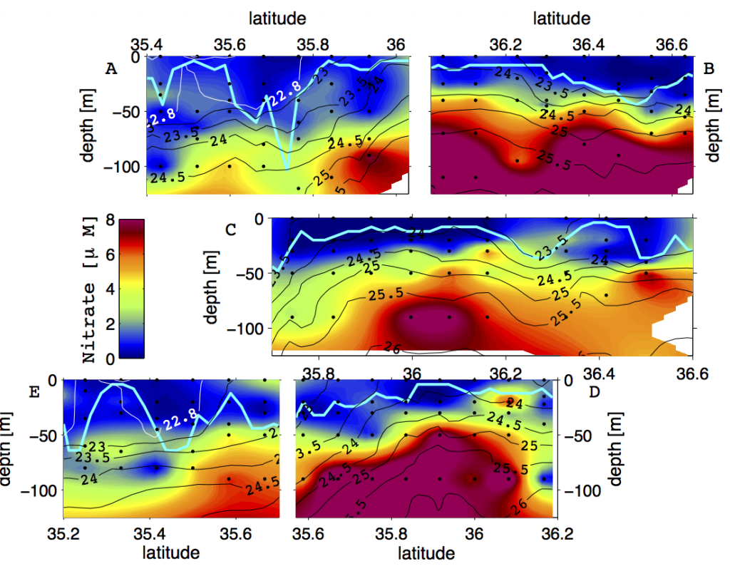
Figure 1. Vertical sections of nitrate (μM) observed across the Kuroshio Extension in October 2009. The panels are organized such that they line up with respect to the density structure of the Kuroshio Extension Front. Cyan contour lines show the mixed layer depth (taken from Nagai and Clayton 2017).
Phytoplankton biomass, community structure, and dynamics
WBCs separate regions with markedly different biogeochemical and ecological characteristics. Subpolar gyres are productive, highly seasonal, tend to support ecosystems with higher phytoplankton biomass, and can be dominated by large phytoplankton and zooplankton taxa. Conversely, subtropical gyres are mostly oligotrophic, support lower photoautotrophic biomass, and are not characterized by a strong seasonal cycle. In turn, these subtropical regions tend to support ecosystems that comprise smaller cells and a tightly coupled microbial loop. As boundaries to these diverse regions, WBCs are the main conduit linking the equatorial and polar oceans and their resident plankton communities. Within the frontal zones, mesoscale dynamics act to stir water masses together and can transport ecosystems across the WBC into regions of markedly different physical and biological characteristics. Furthermore, mesoscale eddies can modulate vertical fluxes via the displacement of ispycnals during eddy intensification or eddy-induced Ekman pumping, or generating submesoscale patches of vertical exchange. At these smaller scales, vigorous vertical circulations ¾ with magnitudes reaching 100 m/day ¾ can fertilize the euphotic zone or transport phytoplankton out of the surface layer.
Numerous studies have hypothesized that the combination of large-scale transport, mesoscale stirring and transport, and submesoscale nutrient input leads to both high biodiversity and high population densities. Using remote sensing data, D’Ovidio et al. (2010) showed that mesoscale stirring in the Brazil-Malvinas Confluence Zone brings together communities from very different source regions, driving locally enhanced biodiversity. In a numerical model, in which physical and biological processes can be explicitly separated and quantified, Clayton et al. (2013) showed that high modeled biodiversity in the WBCs was due to a combination of transport and local nutrient enhancements. And finally, in situ taxonomic surveys crossing the Brazil-Malvinas Confluence (Cermeno et al. 2008) and the Kuroshio Extension (Honjo and Okada 1974; Clayton et al, 2017) showed both enhanced biomass and biodiversity associated with the WBC fronts. Beyond these local enhancements, WBCs might play a larger role in setting regional biogeography. Sugie and Suzuki (2017) found a mixture of temperate and subpolar diatom species in the Kuroshio Extension, suggesting that the boundary current might play a key role in setting downstream diatom diversity.
However tantalizing these results are, they remain relatively inconclusive, in part because of their relatively small temporal and spatial scales. Extending existing approaches for assessing phytoplankton community structure, leveraging emerging ‘omics and continuous sampling techniques, larger regions might be surveyed at high taxonomic and spatial resolution. Combining genomic and transcriptomic observations would provide measures of both organism abundance and activity (Hunt et al. 2013), as well as the potential to better define the relative roles of growth and loss processes. With genetically resolved data and appropriate survey strategies, it will be possible to conclusively determine the presence of these biodiversity hotspots. A better characterization and deeper understanding of these regions will provide insight into the long-term and large-scale biodiversity, stability, and function of the global planktonic ecosystem.
Organic carbon export via physical and biological processes
Export, the removal of fixed carbon from the surface ocean, is driven by gravitational particle sinking, active transport, and (sub)mesoscale processes such as eddy-driven subduction. While evidence suggests that WBCs are likely hot spots of biological (Siegel et al. 2014; Honda et al. 2017a) and physical (Omand et al. 2015) export fluxes out of the euphotic zone, only a small handful of studies have explored this. Recent results from sediment trap studies at the Kuroshio Extension Observatory (KEO) mooring, located just south of the Kuroshio Extension, suggest that there is a link between the passage of mesoscale eddies and carbon export (Honda et al. 2017b). They observed that high export events at 5000 m lagged behind the passage of negative (cyclonic) sea surface height anomalies (SSHA) at the mooring by one to two months (Figure 2). In other regions, underway measurements (Stanley et al. 2010) and optical sensors on autonomous platforms (Briggs et al. 2011; Estapa et al. 2013; Estapa et al. 2015; Bishop et al. 2016) have revealed large episodicity in export proxies over timescales of hours to days and spatial scales of 1-10 km.
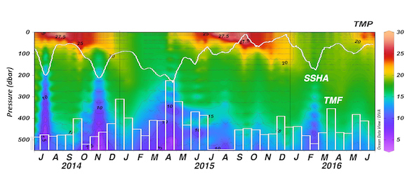
Figure 2. Time series of ocean temperature in the upper ~550 m (less than 550 dbar) at station KEO between July 2014 and June 2016. The daily data shown in the figure are available on the KEO database. White contour lines show the temporal variability in the daily satellite-based sea surface height anomaly (SSHA). White open bars show the total mass flux (TMF) observed by the time series sediment trap at 5000 m (based on a figure in Honda et al. 2017b).
Another avenue of carbon export from the surface ocean results from grazing and vertical migration. Vertically migrating zooplankton feed near the surface in the dark and evade predation at depth during the day. Fronts generated by WBCs produce gradients in zooplankton communities, both in terms of grazer biomass and species compositions (e.g., Wiebe and Flierl, 1983), and influence the extent and magnitude of diel vertical migrations. Submesoscale variability in zooplankton abundance can be observed readily in echograms collected by active acoustic sensors, but submesoscale variability in zooplankton community structure and dynamics remains difficult to measure. Thus, the nature of this variability remains largely unknown.
Future research directions
Building a better understanding of how physical and biogeochemical dynamics in WBC regions interact relies on observing these systems at the appropriate scales. This is particularly challenging because of the range of scales at play in these systems and the limitation of existing in situ and remote observing platforms and techniques. As has been outlined above, the ecological and biogeochemical environment of WBCs is the result of long range transport from the flanking subtropical and subpolar gyres, as well as local modification by meso- and submesocale physical dynamics in these frontal systems.
Another challenge in disentangling the relationships between physical and biogeochemical processes in WBCs is the difficulty in measuring rates rather than standing stocks. In such dynamic systems, lags in biological responses mean that the changes in standing stocks may not be collocated with the physical process forcing them. Small-scale lateral stirring spatially and temporally decouples net community production and export while secondary circulations contribute to vertical transport. As much as possible, future process studies should include approaches that can explicitly quantify biological rates and physical transport pathways. New platforms are beginning to fill these observational gaps: BGC-Argo floats, autonomous platforms (e.g., Saildrone), high-frequency underway measurements, and continuous cytometers (including imaging cytometers) are all capable of generating high-spatial resolution datasets of biological and chemical properties over large regions. Gliders and profiling platforms (e.g., WireWalker) are making it possible to measure vertical profiles of biogeochemical properties at high frequency. Operating within a Lagrangian framework, while resolving lateral gradients of physical and biogeochemical tracers with ships or autonomous vehicles, may someday allow us to quantitatively partition the observed small-scale variability in biogeochemical tracers between that attributable to biological or physical processes.
References
Bishop, J. K. B., M. B. Fong, and T. J. Wood, 2016: Robotic observations of high wintertime carbon export in California coastal waters. Biogeosci., 13, 3109-3129, doi:10.5194/bg-13-3109- 2016.
Briggs, N., M. J. Petty, I. Cetinic, I., C. Lee, E. A. Dasaro, A. M. Gray, and E. Rehm, 2011: High-resolution observations of aggregate flux during a subpolar North Atlantic spring bloom. Deep-Sea Res. I, 58, 10311039, doi:10.1016/j.dsr.2011.07.007.
Cermeno, P., S. Dutkiewicz, R. P. Harris, M. Follows, O. Schofield, and P. G. Falkowski, 2008: The role of nutricline depth in regulating the ocean carbon cycle. Proc. Natl. Acad. Sci., 105, 20344-20349. doi:10.1073/pnas.0811302106.
Clayton, S., S. Dutkiewicz, O. Jahn, and M. J. Follows, 2013: Dispersal, eddies, and the diversity of marine phytoplankton. Limn. Ocean. Fluids Env., 3, 182-197. doi:10.1215/21573689-2373515.
Clayton, S., T. Nagai, and M. J. Follows, 2014: Fine scale phytoplankton community structure across the Kuroshio Front. J. Plankton Res., 36, 1017-1030. doi:10.1093/plankt/fbu020.
Clayton, S., Y.-C. Lin, M. J. Follows, and A. Z. Worden, 2017: Co-existence of distinct Ostreococcus ecotypes at an oceanic front. Limn. Ocean.. 62, 75-88, doi:10.1002/lno.10373.
D’Asaro, E., C. Lee, L. Rainville, L. Harcourt, and L. Thomas, 2011: Enhanced turbulence and energy dissipation at ocean fronts. Science, 332, 318–322, doi: 10.1126/science.1201515.
Estapa, M. L., K. Buesseler, E. Boss, and G. Gerbi, 2013: Autonomous, high-resolution observations of particle flux in the oligotrophic ocean. Biogeosci., 10, 5517-5531, doi: 10.5194/bg-10-5517-2013.
Estapa, M. L., D. A. Siegel, K. O. Buesseler, R. H. R. Stanley, M. W. Lomas, and N. B. Nelson, 2015: Decoupling of net community and export production on submesoscales in the Sargasso Sea. Glob. Biogeochem. Cyc., 29, 12661282, doi:10.1002/2014GB004913.
Guo, X., X.-H. Zhu, Q.-S. Wu, and D. Huang, 2012: The Kuroshio nutrient stream and its temporal variation in the East China Sea. J. Geophys. Res. Oceans, 117, doi:10.1029/2011jc007292.
Guo, X. Y., X. H. Zhu, Y. Long, and D. J. Huang, 2013: Spatial variations in the Kuroshio nutrient transport from the East China Sea to south of Japan. Biogeosci., 10, 6403-6417, doi:10.5194/bg-10-6403-2013.
Honda, M. C., and Coauthors, 2017a: Comparison of carbon cycle between the western Pacific subarctic and subtropical time-series stations: highlights of the K2S1 project. J. Oceanogr., 73, 647-667, doi:10.1007/s10872-017-0423-3.
Honda, M.C., Y. Sasai, E. Siswanto, A. Kuwano-Yoshida, and M. F. Cronin, 2017b: Impact of cyclonic eddies on biogeochemistry in the oligotrophic ocean based on biogeochemical /physical/meteorological time-series at station KEO. Prog. Earth Planet. Sci., submitted.
Honjo, S., and H. Okada, 1974: Community structure of coccolithophores in the photic layer of the mid-Pacific. Micropaleo., 20, 209-230, doi:10.2307/1485061.
Hunt, D. E., Y. Lin, M. J. Church, D. M. Karl, S. G. Tringe, L. K. Izzo, and Z. I. Johnson, 2013: Relationship between abundance and specific activity of bacterioplankton in open ocean surface waters. Appl. Environ. Microbiol., 79, 177-184, doi:10.1128/AEM.02155-12.
Inoue, R., M. C. Gregg, and R. R. Harcourt, 2010: Mixing rates across the Gulf Stream, Part 1: On the formation of Eighteen Degree Water. J. Mar. Res. 68, 643–671.
Kaneko, H., I. Yasuda, K. Komatsu, and S. Itoh, 2012: Observations of the structure of turbulent mixing across the Kuroshio. Geophys. Res. Lett. 39, doi:10.1029/2012GL052419.
Nagai, T., A. Tandon, H. Yamazaki, and M. J. Doubell, 2009: Evidence of enhanced turbulent dissipation in the frontogenetic Kuroshio Front thermocline. Geophys. Res. Lett., 36, doi:10.1029/2009GL038832.
Nagai, T., A. Tandon, H. Yamazaki, M. J. Doubell, and S. Gallager, 2012: Direct observations of microscale turbulence and thermohaline structure in the Kuroshio Front. J. Geophys. Res., 117, doi:10.1029/2011JC007228.
Nagai, T., M. Aiba, and S. Clayton, 2015a: Multiscale route to supply nutrients in the Kuroshio. Kaiyo-to-Seibutsu (In Japanese), 37, 469-477.
Nagai, T., A. Tandon, E. Kunze, and A. Mahadevan, 2015b: Spontaneous generation of near-inertial waves by the Kuroshio Front. J. Phys. Oceanogr., 45, 2381-2406, doi:10.1175/JPO-D-14-0086.1.
Nagai, T., R. Inoue, A. Tandon, and H. Yamazaki, 2015c: Evidence of enhanced double-diffusive convection below the main stream of the Kuroshio Extension. J. Geophys. Res.,120, 8402-8421, doi: 10.1002/2015JC011288.
Nagai, T., and S. Clayton, 2017: Nutrient interleaving below the mixed layer of the Kuroshio Extension Front. Ocean Dyn., 67, 1027-1046, doi:10.1007/s10236-017-1070-3.
Omand, M. M., M. J. Perry, E. D’Asaro, C. Lee, N. A. Briggs, I. Cetinic, and A. Mahadevan, 2015: Eddy-driven subduction exports particulate organic carbon from the spring bloom. Science, 348, 222–225, doi:10.1126/science.1260062.
d’Ovidio, F., S. De Monte, S. Alvain, Y. Dandonneau, and M. Lévy, 2010: Fluid dynamical niches of phytoplankton types. Proc. Natl. Acad. Sci., 107, 18366-18370. doi:10.1073/pnas.1004620107
Pelegrí, J. L., and G. T. Csanady, 1991: Nutrient transport and mixing in the Gulf Stream. J. Geophys. Res. Oceans, 96, 2577-2583, doi:10.1029/90JC02535.
Pelegrí, J. L., G. T. Csanady, and A. Martins, 1996: The North Atlantic nutrient stream. J. Oceanogr., 52, 275-299, doi: 10.1007/BF02235924.
Sarmiento, J. Á., N. Gruber, M. A. Brzezinski, and J. P. Dunne, 2004: High-latitude controls of thermocline nutrients and low latitude biological productivity. Nature, 427, 56-60, doi:10.1038/nature02127.
Siegel, D. A., K. O. Buesseler, S. C. Doney, S. F. Sailley, M. J. Behrenfeld, and P. W. Boyd, 2014: Global assessment of ocean carbon export by combining satellite observations and food‐web models. Glob. Biogeochem. Cycles, 28, 181-196, doi: 10.1002/2013GB004743.
Stanley, R. H. R., J. B. Kirkpatrick, N. Cassar, B. A. Barnett, and M. L. Bender, 2010: Net community production and gross primary production rates in the western equatorial Pacific: Western equatorial Pacific production. Glob. Biogeochem. Cycles, 24, doi:10.1029/ 2009GB003651.
Sugie, K., and K. Suzuki, 2017: Characterization of the synoptic-scale diversity, biogeography, and size distribution of diatoms in the North Pacific. Limnol. Oceanogr., 62, 884-897, doi:10.1002/lno.10473.
Tsutsumi, E., T. Matsuno, R. C. Lien, H. Nakamura, T. Senjyu, and X. Guo, 2017: Turbulent mixing within the Kuroshio in the Tokara Strait. J. Geophys. Res. Oceans, 122, 7082-7094, doi:10.1002/2017JC013049.
Wiebe, P., and G. Flierl, 1983: Euphausiid invasion/dispersal in Gulf Stream cold-core rings. Mar. Fresh. Res., 34, 625–652, doi: 10.1071/MF9830625.
Williams, R. G., V. Roussenov, and M. J. Follows, 2006: Nutrient streams and their induction into the mixed layer. Glob. Biogeochem. Cycles, 20, doi:10.1029/2005gb002586.