mmaheigan :: Ocean Carbon & Biogeochemistry

Studying marine ecosystems and biogeochemical cycles in the face of environmental change

Author Archive for mmaheigan – Page 33

The changing ocean carbon cycle

Posted by mmaheigan

· Thursday, July 6th, 2017

Since preindustrial times, the ocean has removed from the atmosphere 41% of the carbon emitted by human industrial activities (Figure 1). The globally integrated rate of ocean carbon uptake is increasing in response to rising atmospheric CO₂ levels and is expected to continue this trend for the foreseeable future. However, the inherent uncertainties in ocean surface and interior data associated with ocean carbon uptake processes make it difficult to predict future changes in the ocean carbon sink. In a recent paper, McKinley et al. (2017), review the mechanisms of ocean carbon uptake and its spatiotemporal variability in recent decades. Looking forward, the potential for direct detection of change in the ocean carbon sink, as distinct from interannual variability, is assessed using a climate model large ensemble, a novel approach to studying climate processes with an earth systems model, the “large ensemble.” In a large ensemble, many runs of the same model are done so as to directly distinguish natural variability from long-term trends.

This analysis illustrates that variability in CO₂ flux is large enough to prevent detection of anthropogenic trends in ocean carbon uptake on at least decadal to multi-decadal timescales, depending on location. Earliest detection of trends is most attainable in regions where trends are expected to be largest, such as the Southern Ocean and parts of the North Atlantic and North Pacific. Detection will require sustained observations over many decades, underscoring the importance of traditional ship-based approaches and integration of new autonomous observing platforms as part of a global ocean carbon observing system.

Please see a relevant OCB outreach tool on ocean carbon uptake developed by McKinley and colleagues:
OCB teaching/outreach slide deck Temporal and Spatial Perspectives on the Fate of Anthropogenic Carbon: A Carbon Cycle Slide Deck for Broad Audiences – also download explanatory notes

Quantifying coastal and marine ecosystem carbon storage potential for climate mitigation policy and management

Posted by mmaheigan

· Wednesday, June 21st, 2017

Under the increasing threat of climate change, conservation practitioners and policy makers are seeking innovative and data–driven recommendations for mitigating emissions and increasing natural carbon sinks through nature-based solutions. While the ocean and terrestrial forests, and more recently, coastal wetlands, are well known carbon sinks, there is interest in exploring the carbon storage potential of other coastal and marine ecosystems such as coral reefs, kelp forests, phytoplankton, planktonic calcifiers, krill, and teleost fish. A recent study in Frontiers in Ecology and the Environment reviewed the potential and feasibility of managing these other coastal and marine ecosystems for climate mitigation. The authors concluded, that while important parts of the carbon cycle, coral reefs, kelp forests, planktonic calcifiers, krill, and teleost fish do not represent long-term carbon stores, and in the case of fish, do not represent a sequestration pathway. Phytoplankton do sequester globally significant amounts of carbon and contribute to long-term carbon storage in the deep ocean, but there is currently no good way to manage them to increase their carbon storage capacity; additionally, the vast majority of phytoplankton is located in international waters that are outside national jurisdictions, making it very difficult to include them in current climate mitigation policy frameworks.

Comparatively, coastal wetlands (mangroves, tidal marshes, and seagrasses) effectively sequester carbon long-term (up to 10x more carbon stored per unit area than terrestrial forests with 50-90% of the stored carbon residing in the soil), and fall within clear national jurisdictions, which facilitates effective and quantifiable management actions. In addition, wetland degradation has the potential to release vast amounts of stored carbon back into the atmosphere and water column, meaning that conservation and restoration of these systems can also reduce potential emissions. The authors conclude that coastal wetland protection and restoration should be a primary focus in comprehensive climate change mitigation plans along with reducing emissions.

Authors:
Jennifer Howard (Conservation International)
Ariana Sutton-Grier (University of Maryland, NOAA)
Dorothée Herr (IUCN)
Joan Kleypas (NCAR)
Emily Landis (The Nature Conservancy)
Elizabeth Mcleod (The Nature Conservancy)
Emily Pidgeon (Conservation International)
Stefanie Simpson (Restore America’s Estuaries)

Original paper: http://onlinelibrary.wiley.com/doi/10.1002/fee.1451/full

Winter ventilation depth constrains the impact of the biological pump on CO2 uptake in the North Pacific Ocean

Posted by mmaheigan

· Thursday, June 8th, 2017

The North Pacific accounts for ~25% of the global ocean’s uptake of carbon dioxide (CO₂) from the atmosphere. However, the relative importance of the biological pump vs. physical circulation in driving ocean uptake of CO₂ remains poorly understood.

In a recent study, Palevsky and Quay (2017) used geochemical measurements collected on sixteen container ship transects between Hong Kong and Long Beach, CA to evaluate the drivers of CO₂ uptake across 8,000 kilometers in the North Pacific basin over the full annual cycle. In the eastern North Pacific, biologically-driven export of organic carbon below the winter ventilation depth fully offsets the uptake of CO₂ from the atmosphere. However, in the Kuroshio region of the western North Pacific, which has a deep winter mixed layer, the majority of the organic carbon exported during the productive summer season is subsequently respired and ventilated back to the atmosphere in winter. Subsequently, biologically-driven export offsets only a small fraction of the CO₂ uptake by the ocean and, instead, physical transport is the dominant process removing inorganic carbon from the region.

We further show that that mechanistic coupling between biological carbon export and ocean uptake of CO₂ from the atmosphere is sensitive to the seasonal timing of biological export and ventilation, as well as the magnitude of export. Future studies therefore need to measure biological carbon export and ventilation throughout the full annual cycle in order to better understand controls on regional variations in ocean CO₂ uptake rates and future changes in these rates.

Data from 16 shipboard transects across the North Pacific revealed a basin-wide gradient between the Kuroshio and Eastern regions in the relative roles of biological vs. physical processes in removing dissolved inorganic carbon from the surface ocean.

Authors:
Hilary I. Palevsky (Woods Hole Oceanographic Institution)
Paul D. Quay (University of Washington)

OCB supports early career participation in 3rd International Ocean Colour Science Meeting

Posted by mmaheigan

· Tuesday, June 6th, 2017

OCB-sponsored participants of 3rd International Ocean Color Meeting in May 2017.

Christiana Ade is a first-year PhD student at North Carolina State University in the Marine, Earth and Atmospheric Sciences Department. She researches wetlands and coastal environments using satellite remote sensing and field measurements. Her research includes water quality mapping, establishing new environmental indicators, and determining satellite resolution requirements for adequately monitoring wetlands.

“As a master’s student, I focused on wetland vegetation, but for my PhD I am shifting toward water quality monitoring. The 2017 IOCS meeting occurred at a critical time in my career as I begin this research transition. IOCS allowed me to meet several prominent researchers and advanced students that I foresee myself collaborating with in the future, thus furthering my long-term objective of becoming a researcher in a national lab or university professor. I presented a poster at IOCS on some preliminary research and received extremely useful feedback, which I am already implementing. Although the conference was great for networking, it was most beneficial for expanding my understanding of current limitations and future opportunities in remote sensing of water. In particular, the breakout sessions provided me with several insights on hot-button topics and gave me confidence that the ocean color community will aid researchers invested in coastal applications to determine what sensor resolutions are needed to monitor these environments. Meetings like this ensure that the necessary technology gets built and launched. I would like to thank all the organizers, speakers, and the OCB for their positive impact on my research career.”

Henry Houskeeper is a third year Ocean Sciences PhD student working with Raphael Kudela at the University of California, Santa Cruz. Henry investigates the optical properties of dinoflagellate red tides. His broader interests include remote sensing of the coastal ocean, coastal upwelling ecosystem dynamics, and phytoplankton ecology.

“Attending the IOCS meeting was an excellent opportunity for me to receive thoughtful feedback on my research. IOCS connected me with helpful members of the ocean color community and exposed me to a diverse assemblage of ocean color research projects. The support from OCB made this valuable experience possible for me.”

Suhey Ortiz Rosa is a PhD student conducting research with Dr. Roy Armstrong in Bio-Optical Oceanography at the Department of Marine Sciences at the University of Puerto Rico- Mayagüez (UPRM). In 2005, she completed a B.S. in Coastal Marine Biology at the University of Puerto Rico- Humacao, and in 2010, a MS in Chemical Oceanography at UPRM. Suhey’s work focuses on the biogeochemistry of coastal waters and coral reefs, validating algorithms from satellite imagery of complex optical waters, remote sensing, and GIS. Previously, she worked on CDOM characterization with PARAFAC, mapping marine species distribution with the GAP-Analysis Project of Puerto Rico and later with watershed analysis of sedimentation processes on coral reefs.

“The International Ocean Color Science Meeting was a unique experience. Networking with the international community to address common issues on satellite imagery analysis benefits my research tremendously. I am now able to communicate with leading experts that work with the latest processes, allowing me to conduct more accurate and efficient research. The workshop on Copernicus Data was also very helpful, providing hands-on personalized experience. The cultural diversity and different research projects presented made this conference an advantage for me as an early career ocean color researcher. The information I obtained expands my options for new opportunities and ideas in research. It is fundamental for young scientists to remain up to date with the innovations in their current research topic. Thanks to the OCB program for making this experience possible!”

Sara Rivero-Calle is a postdoctoral researcher at the Levine Lab in the University of Southern California interested in projects that involve large datasets, combining remote sensing and in situ data to answer large-scale ecological questions. She first learned about satellite remote sensing during her MS program at the University of Puerto Rico working on mesophotic reef sponge ecology using Autonomous Underwater Vehicles. She earned a PhD from Johns Hopkins University, where she used the Continuous Plankton Recorder survey to study long-term changes in North Atlantic phytoplankton communities. Currently, Sara is conducting postdoctoral research on fine-scale variability and patchiness, combining remote sensing, float, and HPLC data with numerical models.

“Attending IOCS was a fantastic experience. I was invited to give a talk on the global distribution of Trichodesmium for the special session on Trichodesmium. This was a great opportunity, not only for the exposure, but also because I am now collaborating with the organizers on writing a white paper with recommendations for remote sensing of Trichodesmium from space. This is perfect timing, given the new sensors with higher spatial and spectral resolution currently being developed and forthcoming satellite missions. I also noticed a clear interest in the remote sensing community to work closely with modelers and I think I can help bridge the two communities. I will be collaborating with another working group focused on carbon cycling. One of the things I liked most was the IOCS meeting structure—splitting us up into working groups, identifying current challenges and brainstorming together on how to deal with them and move forward. This meeting is not focused on presenting work but on setting new goals and working towards them. I also liked that the IOCS meeting facilitates direct communication with program managers and representatives from all space agencies and how the agencies came to the meeting to hear what the scientific community needs to advance satellite remote sensing. In summary, the IOCS meeting is the perfect venue for international scientific networking and I am so grateful to OCB for supporting us at an early stage of our career, thanks for believing in us!”

Sarah Schlunegger is a PhD Student in the Program of Atmospheric and Oceanic Sciences, advised by Prof. Jorge Sarmiento. Sarah uses Earth System Models to predict the timing, sequence and inter-dependence of emerging anthropogenic signals in the ocean, with a focus on the ocean’s acquisition of anthropogenic carbon and heat. The ocean provides a climate service by absorbing the atmosphere’s excess carbon and heat but at a cost, namely acidification and warming, which deteriorate marine habitats. Sarah’s primary research goal is to identify when and where changes in these heat/carbon sinks and their resulting impacts will be detectable in the ocean.

“As a climate modeler, I have limited daily interactions with observationalists, despite my using satellite observations as a component of my own research. The 2017 International Ocean Colour Science Meeting was the perfect platform to cure this condition! Hearing talks and discussion from the lead scientist and engineers who have spent decades developing and perfecting satellite observation platforms has expanded my understanding and appreciation for the work behind the end-product. I enjoyed listening to the expert panels parse through upcoming innovations to address atmospheric correction, a major challenge faced by the community. The fellow conference attendees were friendly and encouraging, and of course, Lisbon is a magical city!”

Do rivers supply nutrients to the open ocean?

Posted by mmaheigan

· Wednesday, May 24th, 2017

Rivers carry large amounts of nutrients (e.g., nitrogen and phosphorus) to the sea, but we do not know how much of that riverine nutrient supply escapes biological and chemical processing in shallow coastal waters to reach the open ocean. Most global ocean biogeochemical models, which are typically unable to resolve coastal processes, assume that either all or none of the riverine nutrients entering coastal waters actually contribute to open ocean processes.

While we know a good deal about the dynamics of individual rivers entering the coastal ocean, studies to date have been limited to a few major river systems, mainly in in developed countries. Globally, there are over 6,000 rivers entering the coastal ocean. In a recent study, Sharples et al (2017) devised a simple approach to obtain a global-scale estimate of riverine nutrient inputs based on the knowledge that low-salinity waters entering the coastal ocean tend to form buoyant plumes that turn under the influence of Earth’s daily rotation to flow along the coastline. Using published data on such flows and incorporating the effect of Earth’s rotation, they obtained estimates of typical cross-shore plume width and compared them to the local width of the continental shelf. This was used to calculate the residence time of riverine nutrients on the shelf, which is the key to estimating how much of a given nutrient is consumed in shelf waters vs. how much is exported to the open ocean.

Global distribution of the amount of riverine dissolved inorganic nitrogen that escapes the continental shelf to reach the open ocean.

The results indicate that, on a global scale, 75% (80%) of the nitrogen (phosphorus) supplied by rivers reaches the open ocean, whereas 25% (20%) of the nitrogen (phosphorus) is consumed on the shelf (e.g., fueling coastal productivity). Limited knowledge of nutrient cycling and consumption in shelf waters represents the primary source of uncertainty in this study. However, well-defined global patterns related to human land use (e.g., agricultural fertilizer use in developed nations) emerged from this analysis, underscoring the need to understand how land-use changes and other human activities will alter nutrient delivery to the coastal ocean in the future.

Authors:
Jonathan Sharples (School of Environmental Sciences, University of Liverpool, UK)
Jack Middelburg (Department of Earth Sciences, Utrecht University, Netherlands)
Katja Fennel (Department of Oceanography, Dalhousie University, Canada)
Tim Jickells (School of Environmental Sciences, University of East Anglia, UK)

A Training Course on Marine Radioactivity August 13, 2017

Posted by mmaheigan

· Monday, May 15th, 2017

A Training Course on Marine Radioactivity in association with Goldschmidt, August 13, 2017. The event, organized by SCOR 146 WG, will include: An introduction to Radionuclides, Natural, Anthropogenic, and Cosmogenic Radioisotopes and their General Applications in the Marine environment, and Radioecology. Specific lectures will delve more deeply into specific applications and include topics such as applications of radionuclides to sediment age dating, submarine groundwater discharge, and biological mediated carbon export.

Lecturers:

Dr. Ken Buesseler, Center for Marine and Environmental Radioactivity, Woods Hole Oceanographic Institution, USA
Dr. Minhan Dai, State Key Laboratory of Marine Environmental Science, Xiamen University, China
Dr. Claudia Benitez‐Nelson, University of South Carolina, USA
Dr. Sabine Charmasson, ISRN, Laboratory for Research on Transfers in the Environment, France
Dr. Pere Masque, Edith Cowan University (Australia) and Universitat Autònoma de Barcelona (Catalonia, Spain)
Dr. Willard S. Moore, University of South Carolina, USA
Dr. John Smith, Bedford Institute of Oceanography, Dartmouth, NS, Canada

Detailed agenda and more information

The course is open to 25 students and early career scientists interested in radiochemisty‐related fields.

Please use the Goldschmidt registration form to register for this workshop and for the Goldschmidt meeting. The workshop registration fee (40 Euros) will be supported in large part by the Center for Marine and Environmental Radioactivity at WHOI.

Scientists reveal major drivers of aragonite saturation state in the Gulf of Maine, a region vulnerable to acidification

Posted by mmaheigan

· Thursday, May 11th, 2017

The Gulf of Maine (GoME) is a shelf region that is especially vulnerable to ocean acidification (OA). GoME’s shelf waters display the lowest mean pH, aragonite saturation state (Ω-Ar), and buffering capacity of the entire U.S. East Coast. These conditions are a product of many unique characteristics and processes occurring in the GoME, including relatively low water temperatures that result in higher CO₂ solubility; inputs of fresher, low-alkalinity water that is traceable to the rivers discharging into the Labrador Sea to the north, as well as local inputs of low-pH river water; and its semi-enclosed nature (long residence time >1 year), which enables the accumulation of respiratory products, i.e. CO₂.

A recent study by Wang et al. (2017) is the first to assess the major oceanic processes controlling seasonal variability of aragonite saturation state and its linkages with pteropod abundance in the GoME. The results indicate that surface production was tightly coupled with remineralization in the benthic nepheloid layer during highly productive seasons, resulting in occasional aragonite undersaturation. Mean water column Ω-Ar and abundance of large thecosomatous pteropods show some correlation, although discrete cohort reproductive success likely also influences their abundance. Photosynthesis-respiration is the primary driving force controlling Ω-Ar variability over the seasonal cycle. However, calcium carbonate (CaCO₃) dissolution appears to occur at depth in fall and winter months when bottom water Ω-Ar is generally low but slightly above 1. This is accompanied by a decrease in pteropod abundance that is consistent with previous CaCO₃ flux trap measurements.

Figure. Changes of aragonite saturation states (ΔΩ) between three consecutive cruises from April – July 2015 as a function of changes in salinity-normalized DIC (ΔenDIC, including correction of freshwater inputs) (a) and changes in salinity-normalized TA (ΔenTA, including correction of freshwater inputs) (b). The data points circled in (b) represent potential alkalinity sources from CaCO3 dissolution and/or anaerobic respiration. Solid lines are theoretical lines of ΔΩ vs. ΔenDIC and ΔΩ vs. ΔenTA expected if only photosynthesis and respiration/remineralization occur. Dashed lines are theoretical lines if only calcification and dissolution of CaCO3 occur.

Under the current rate of OA, the mean Ω-Ar of the subsurface and bottom waters of the GoME will approach undersaturation (Ω-Ar < 1) in 30-40 years. As photosynthesis and respiration are the major driving mechanisms of Ω-Ar variability in the water column, any biological regime changes may significantly impact carbonate chemistry and the GoME ecosystem, including the CaCO₃ shell-building capacity of organisms that are critical to the GoME food web.

Author:

Zhaohui Aleck Wang (Woods Hole Oceanographic Institution)

Biophysical drivers of vigorous carbon cycling near the Kuroshio Extension

Posted by mmaheigan

· Thursday, April 27th, 2017

The Kuroshio Current and its Extension jet in the western North Pacific Ocean form a dynamic western boundary current (WBC) region characterized by large air-sea exchanges of heat and carbon dioxide gas (CO₂). The jet is known to oscillate between stable and meandering states on multi-year timescales that alter the eddy field and depth of winter mixing in the southern recirculation gyre. These dynamic state changes have been shown to imprint biogeochemical signatures onto regional mode waters that can be distributed widely throughout the North Pacific and remain out of contact with the atmosphere for decades.

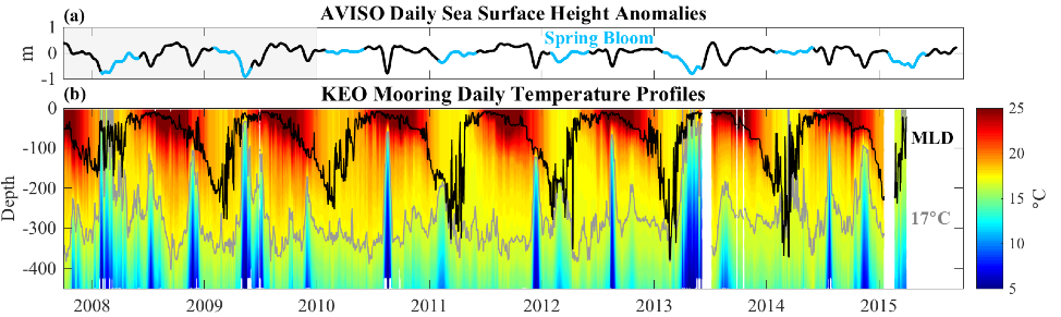
Figure. ~7 years of (a) AVISO daily sea surface height (SSH) anomalies and (b) upper-ocean temperature from the NOAA Kuroshio Extension Observatory (KEO) surface mooring. Black and gray lines in b show the mixed layer depth (MLD) and 17C contour, respectively. Spring bloom periods are indicated in blue in a. The semi-regular upwelling of cold water and corresponding depression of SSH is caused by cold-core eddies that pass the KEO mooring. Winter ventilation depths increase by ~100 m after 2010 when the extension jet entered a stable phase.

To better characterize carbon cycling in this region, ~7 years of daily-averaged autonomous CO₂ observations from NOAA’s Kuroshio Extension Observatory (KEO) surface mooring were used to close the mixed layer carbon budget. High rates of net community production (NCP; >100 mmol C m^-2 d^-1) were observed during the spring bloom period, and a mean annual NCP of 7±3 mol C m^-2 yr^-1 was determined. Biological processes near KEO largely balance the input of carbon that occurs annually through winter mixing; however, physical processes that deviate from climatology were not resolved in this study. Therefore, it remains unclear how transient features such as eddies influence biological carbon production and export through altered nutrient supply and active vertical transport of organic material. Further work is required to determine how biophysical interactions during mesoscale and submesoscale disturbances contribute to local carbon cycle processes and variability in regional mode water carbon inventories.

Ocean Carbon Hot Spots, an upcoming workshop focused on understanding biophysical drivers of carbon uptake in WBC regions, will be held September 25-26, 2017 at the Monterey Bay Aquarium Research Institute (MBARI) in Moss Landing, California. The primary objective of the workshop is to develop a community of observationalists and modelers working on the topic, and to identify critical observational needs that would improve model parameterizations. Ocean Carbon Hot Spots will be co-sponsored by US CLIVAR, US OCB, MBARI, and OMIX.

Written by Andrea J. Fassbender, Monterey Bay Aquarium Research Institute

Mixed-layer carbon cycling at the Kuroshio Extension Observatory (Global Biogeochemical Cycles)

Authors:
Andrea J. Fassbender (Monterey Bay Aquarium Research Institute)
Christopher L. Sabine (NOAA Paciﬁc Marine Environmental Laboratory)
Meghan F. Cronin (NOAA Paciﬁc Marine Environmental Laboratory)
Adrienne J. Sutton (Joint Institute for the Study of the Atmosphere and Ocean, University of Washington)

Satellite Laser Lights Up Polar Research

Posted by mmaheigan

· Thursday, April 13th, 2017

What controls annual cycles and interannual changes in polar phytoplankton biomass? Answers to this question are now emerging from a satellite light detection and ranging (lidar) sensor, which can observe the polar oceans throughout the extensive periods when measurements from traditional passive ocean color sensors are impossible. The new study uses active lidar measurements from the CALIOP satellite sensor to construct complete decade-long record of phytoplankton biomass in the northern and southern polar regions. Results of the study show that annual cycles in biomass are driven by rates of acceleration and deceleration in phytoplankton division, with bloom termination coinciding with maximum division rates irrespective of whether nutrients are exhausted. The study further shows that interannual differences in bloom strength can be quantitatively related to the difference between the winter minimum to summer maximum in division rates. Finally, the analysis indicated that ecological processes had a greater impact than ice cover changes on integrated polar zone phytoplankton biomass in the north, whereas ice cover changes were the dominant driver in the south polar zone. Despite being designed for atmospheric research, CALIOP has provided the first demonstration that active satellite lidar measurements can yield important new insights on plankton ecology in the climate sensitive polar regions. This proof-of-concept creates a foundation for a future ocean-optimized sensor with water-column profiling capabilities that would launch a new lidar era in satellite oceanography.

Authors:

Michael J. Behrenfeld (Oregon State Univ.)
Yongxiang Hu (NASA Langley Research Center)
Robert T. O’Malley (Oregon State Univ.)
Emmanuel S. Boss (Univ. Maine)
Chris A. Hostetler (NASA Langley Research Center)
David A. Siegel (Univ. California Santa Barbara)
Jorge Sarmiento (Princeton Univ.)
Jennifer Schulien (Oregon State Univ.)
Johnathan W. Hair (NASA Langley Research Center)
Xiaomei Lu (NASA Langley Research Center)
Sharon Rodier (NASA Langley Research Center)
Amy Jo Scarino (NASA Langley Research Center)

International team of researchers reports ocean acidification is spreading rapidly in the western Arctic Ocean

Posted by mmaheigan

· Thursday, March 30th, 2017

The Arctic Ocean is particularly sensitive to climate change and ocean acidification such that aragonite saturation state is expected to become undersaturated (Ω_arag <1) there sooner than in other oceans. However, the extent and expansion rate of ocean acidification (OA) in this region are still unknown.

In the March 2017 issue of Nature Climate Change, Qi et al. show that, between 1994 and 2010, low Ω_arag waters have expanded northwards at least 5º, to 85ºN, and deepened from 100 m to 250 m depth. Data from multiple trans-western Arctic Ocean cruises show that Ω_arag<1 water has increased in the upper 250 m from 5 to 31% of the total area north of 70ºN. Tracer data and model simulations suggest that increased transport of Pacific Winter Water (which is already acidified due to both natural and anthropogenic sources), driven by sea-ice retreat and the circulation changes, are primarily responsible for the expansion, while local carbon recycling and anthropogenic CO₂ uptake have also contributed. These results indicate more rapid acidification is occurring in the Arctic Ocean, two to four times faster than the Pacific and Atlantic Oceans, with the western Arctic Ocean the first open-ocean region with large-scale expansion of “acidified” water directly observed in the upper water column.

The rapid spread of ocean acidification in the western Arctic has implications for marine life, particularly clams, mussels and pteropods that may have difficulty building or maintaining their shells in increasingly acidified waters. The pteropods are part of the Arctic food web and important to the diet of salmon and herring. Their decline could affect the larger marine ecosystem.

Authors:
Richard A. Feely (NOAA Pacific Marine Environmental Laboratory)
Leif G. Anderson (Univ. of Gothenburg)
Heng Sun (SOA Third Institute of Oceanography)
Jianfang Chen (SOA Second Institute of Oceanography
Min Chen (Univ. of Delaware)
Liyang Zhan (SOA Third Institute of Oceanography)
Yuanhui Zhang (SOA Third Institute of Oceanography)
Wei-Jun Cai (Univ. of Delaware, Univ. of Georgia)

Funding for the Ocean Carbon & Biogeochemistry Project Office is provided by the National Science Foundation (NSF) and the National Aeronautics and Space Administration (NASA). The OCB Project Office is housed at the Woods Hole Oceanographic Institution.

Author Archive for mmaheigan – Page 33

FilterbyKeyword