The El Niño–Southern Oscillation (ENSO) is a dominant driver of interannual variability in the physical and biogeochemical state of the northeast Pacific, and, consequently, exerts considerable control over the ecological dynamics of the California Current System (CCS). In the CCS, upwelling is the proximate driver of elevated biological production, as it delivers nutrients to the sunlit surface layer of the ocean, stimulating growth of phytoplankton that form the base of the marine food web. Much of the ecosystem variability in the CCS can, therefore, be attributed to changes in bottom-up forcing, which regulates biogeochemical dynamics through a range of mechanisms. Of particular relevance to ENSO-driven variability are the influences of surface winds (which drive upwelling and downwelling), remote oceanic forcing by coastal wave propagation, and alongshore advection. While the relative importance of these individual forcing mechanisms has long been a topic of study, there is general consensus on the qualitative nature of each, and we discuss them in turn below.
Wind
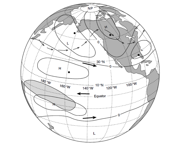
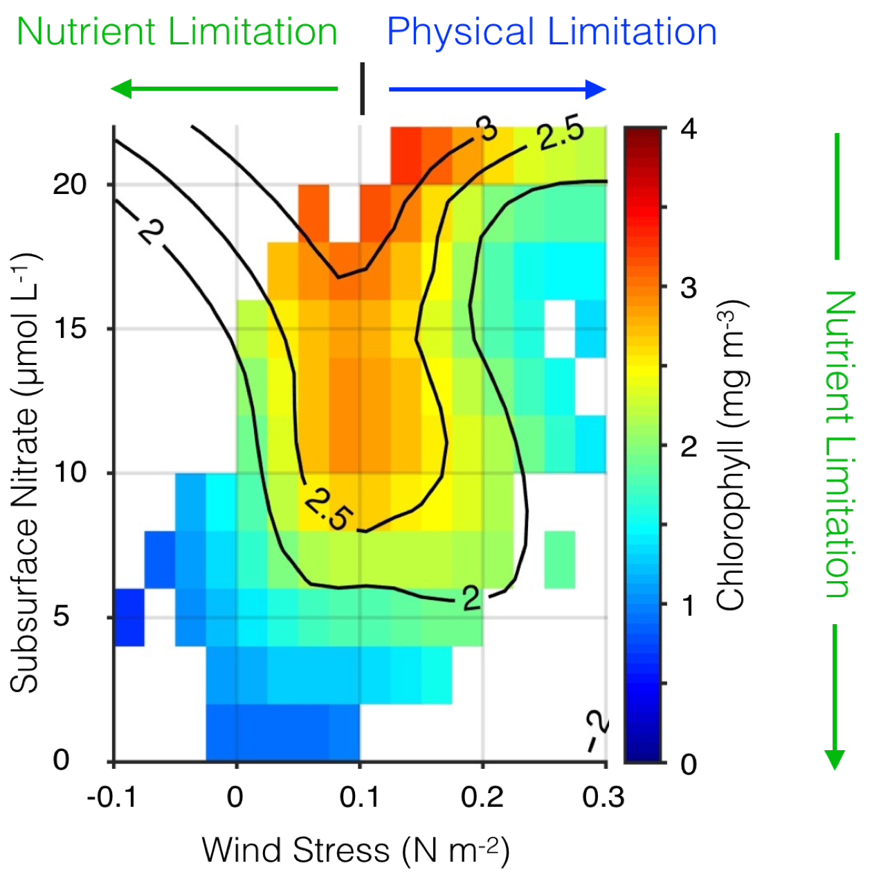
One of the canonical mechanisms by which ENSO events generate an oceanographic response in the CCS is through modification of the surface winds and resultant upwelling. During El Niño, tropical convection excites atmospheric Rossby waves that strengthen and displace the Aleutian low, producing anomalously weak equatorward (or strong poleward) winds, which in turn drive anomalously weak upwelling (or strong downwelling) through modification of cross-shore Ekman transport near the surface (Alexander et al. 2002; Schwing et al. 2002). The opposite response is associated with La Niña. This tropical-extratropical communication through the atmosphere has been given the shorthand name “atmospheric teleconnection.” When equatorward winds are anomalously weak, as they were for example during the 2009-2010 El Niño (Todd et al. 2011), there is a twofold impact on the nutrient flux to the euphotic zone and, consequently, the potential primary productivity. First, weaker winds produce weaker coastal upwelling; independent of changes in the nutrient concentration of upwelling source waters, a reduction in vertical transport translates directly to a reduction in vertical nutrient flux. Second, the nutrient concentration of source waters is altered by the strength of the wind; weak upwelling draws from shallower depths than strong upwelling, and the water that is upwelled is relatively nutrient-poor. Both of these effects tend to limit potential productivity during El Niño. Conversely, La Niña events are associated with anomalously strong equatorward winds, vigorous coastal upwelling, and an ample supply of nutrients to the euphotic zone. However, winds that are too strong can also export nutrients and plankton rapidly offshore, resulting in relatively low phytoplankton biomass in the nearshore region (Figure 1; Jacox et al. 2016a).
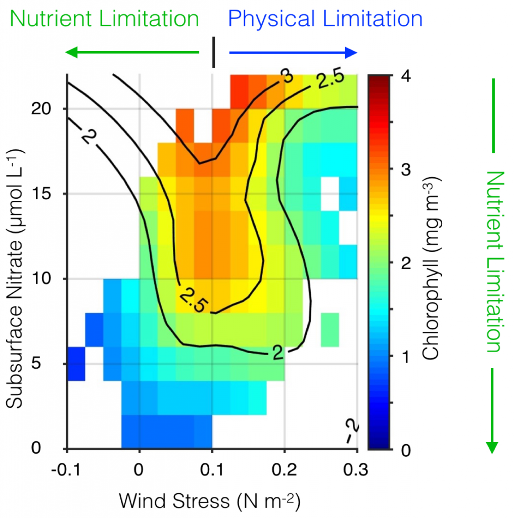
Figure 1. Surface chlorophyll plotted as a function of alongshore wind stress and subsurface nitrate concentration in the central CCS. Wind stress is from the UC Santa Cruz Regional Ocean Model System (ROMS) CCS reanalysis (oceanmodeling.ucsc.edu); nitrate comes from the CCS reanalysis combined with a salinitytemperature-nitrate model developed with World Ocean Database data; and chlorophyll is from the SeaWiFS ocean color sensor. Surface chlorophyll is highest when winds are moderate and subsurface nutrient concentrations are high. Phytoplankton biomass can be hindered by weak upwelling, nitrate-poor source waters, or physical processes (subduction or rapid offshore advection of nutrients and/or phytoplankton, light limitation due to a deep mixed layer) driven by strong winds. Adapted from Jacox et al. (2016a).
In addition to the magnitude of alongshore wind stress, its spatial structure is also important in dictating the ocean’s physical and biogeochemical response. Off the US West Coast, the first mode of interannual upwelling variability is a cross-shore dipole, where anomalously strong nearshore upwelling (within ~50 km of the coast) is accompanied by anomalously weak upwelling farther offshore (Jacox et al. 2014). In terms of the surface wind field, this pattern represents a fluctuation between cross-shore wind profiles with (i) weak nearshore winds and a wide band of positive wind stress curl, and (ii) strong nearshore winds and a narrow band of positive curl. The former, which is associated with positive phases of the Pacific Decadal Oscillation (PDO) and ENSO and negative phases of the North Pacific Gyre Oscillation (NPGO), may favor smaller phyto- and zooplankton, while the latter, associated with negative phases of the PDO and ENSO and positive phases of the NPGO, may favor larger phyto- and zooplankton (Rykaczewski and Checkley 2008).
Remote ocean forcing
As the atmospheric teleconnection transmits tropical variability to CCS winds, an oceanic teleconnection exists in the form of coastally trapped waves that propagate poleward along an eastern ocean boundary and thus approach the CCS from the south (Enfield and Allen 1980; Meyers et al. 1998; Strub and James 2002). During an El Niño, these waves tend to deepen the pycnocline and nutricline, which renders upwelling less effective at drawing nutrients to the surface and, therefore, limits potential productivity. While coastally trapped waves that reach the CCS may originate as far away as the equator, topographic barriers exist, notably at the mouth of the Gulf of California (Ramp et al. 1997; Strub and James 2002) and at Point Conception. Since coastally trapped waves that reach a particular location in the CCS can be generated by wind forcing anywhere along the coast equatorward of that location, the oceanic teleconnection may be thought of as an integration of wind forcing experienced along the equator and all the way up the coast to the CCS. Efforts to separate the effects of local wind forcing from coastally trapped waves are complicated by the strong correlation of alongshore wind along the coast, the fast poleward propagation speed of coastally trapped waves, and the fact that both produce similar effects during canonical El Niño and La Niña events. The 2015-16 El Niño is one example in which warm water and deep isopycnals were observed in the southern CCS despite anomalous local upwelling-favorable winds (Jacox et al. 2016b). In this case, the local winds may have dampened the influence of the oceanic teleconnection (Frischknecht et al. 2017).
Coastally trapped waves are also likely important in setting up an alongshore pressure gradient. The barotropic alongshore pressure gradient influences local upwelling dynamics, as it is balanced primarily by the Coriolis force associated with onshore flow (Connolly et al. 2014). This onshore geostrophic flow acts in opposition to the wind-driven offshore Ekman transport, such that net offshore transport (and consequently upwelling) is less than the Ekman transport (Marchesiello and Estrade 2010). The magnitude of the alongshore pressure gradient is positively correlated with ENSO indices, so it tends to further reduce upwelling during El Niño events, exacerbating the influence of anomalously weak equatorward winds (Jacox et al. 2015).
Alongshore transport
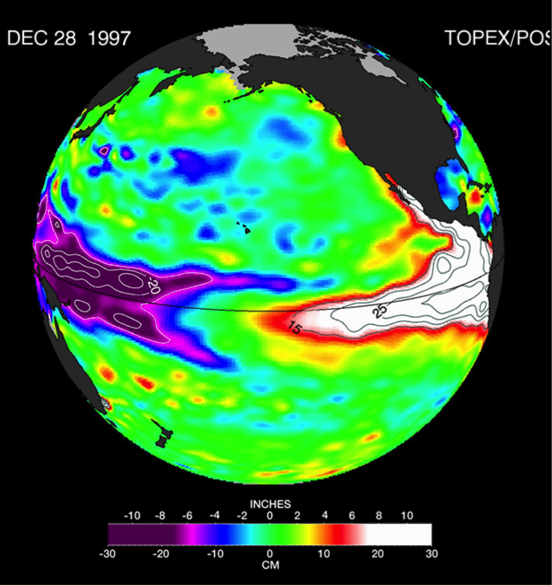
Anomalous alongshore transport has on several occasions been implicated in major ecosystem changes in the CCS. In the case of anomalous advection from the north, as observed in 2002 (Freeland et al. 2003), the CCS is supplied by cold, fresh, and nutrient-rich subarctic water that can stimulate high productivity, even in the absence of strong upwelling. Conversely, anomalous advection of surface waters from the south, as observed during the 1997-98 El Niño (Bograd and Lynn 2001; Lynn and Bograd 2002; Durazo and Baumgartner 2002) may amplify surface warming and water column stratification, intensifying nutrient limitation and biological impacts associated with the atmospheric and oceanic teleconnections.
The poleward flowing California Undercurrent (CUC) may also be modulated by ENSO variability. In particular, there is evidence that strong El Niño events can intensify the CUC (Durazo and Baumgartner 2002; Lynn and Bograd 2002; Gomez-Valdivia et al. 2015), which transports relatively warm, salty, and nutrient-rich water along the North American coast from the tropical Pacific as far north as Alaska (Thomson and Krassovski 2010). Anomalously warm salty water was observed on subsurface isopycnals in the southern CUC during 2015-2016 (Rudnick et al. 2016), suggesting anomalous advection from the south. It is unclear whether coastal upwelling can reach deep enough during El Niño events to draw from the CUC, but if so, the CUC intensification could be a mechanism for modifying upwelling source waters and partially mitigating the previously described impacts on nutrient supply.
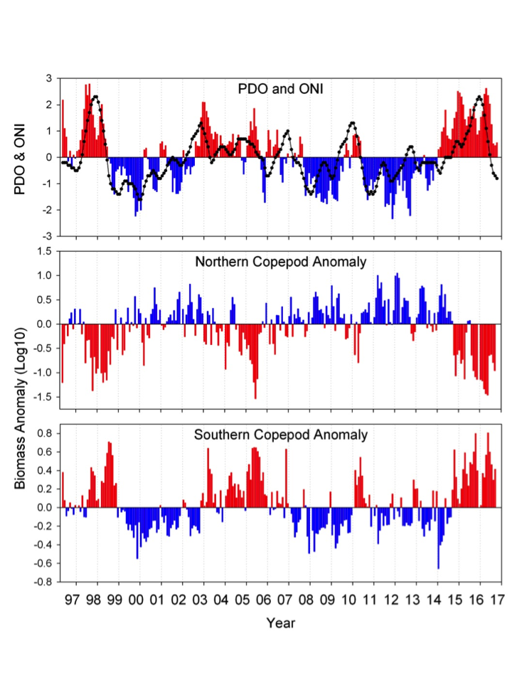
Finally, in addition to influencing the ecosystem through bottom-up forcing, anomalous surface and subsurface currents can directly influence the ecological landscape by transporting species into the CCS from the north, south, or west. For example, positive phases of ENSO and the PDO are associated with higher biomass of warm-water ‘southern’ copepods, while negative phases of ENSO and the PDO are associated with increases in cold-water ‘northern’ copepods (Hooff and Peterson 2006). Importantly, northern copepods are much more lipid-rich than southern copepods; thus, changes in the copepod composition alter the energy available to higher trophic levels and have been implicated in changing survival for forage fish, salmon, and seabirds (Sydeman et al. 2011). During El Niño events, the appearance of additional warm water species (e.g., pelagic red crabs) off the California coast has also been attributed to anomalous poleward advection, though further research is needed to support this hypothesis.
Measuring ENSO’s physical impact on the CCS
While El Niño and La Niña events have specific global and regional patterns associated with them, each ENSO event is unique, both in its evolution and its regional impacts (Capotondi et al. 2015), exemplified by events of the past several years. The tropical evolution of the 2015-16 El Niño was reasonably well predicted by climate models (L’Heureux et al. 2016), in contrast to 2014-15 when a predicted El Niño failed to materialize (McPhaden 2015). However, even in the strong 2015-16 El Niño there were notable exceptions from the expected effects of a strong El Niño, including a lack of increased precipitation over the Southwestern and South Central United States (L’Heureux et al. 2016). Similarly, subsurface ocean anomalies off Central and Southern California were weaker in 2015-16 than they were during the 1982-83 and 1997-98 El Niños (Jacox et al. 2016b), and the 2015-16 El Niño occurred against a backdrop of widespread pre-existing anomalous conditions in the northeast Pacific.
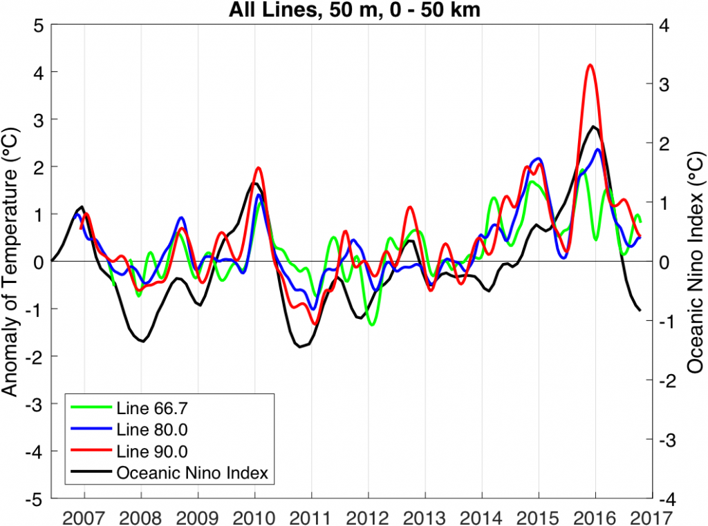
Figure 2. Temperature anomaly at 50 m depth from the California Underwater Glider Network, averaged over the inshore 50 km and filtered with a 3-month running mean. Lines have traditional CalCOFI designations 66.7 (Monterey Bay), 80.0 (Point Conception), and 90.0 (Dana Point). The Oceanic Niño Index (a 3-month running mean of the Niño 3.4 SST anomaly) is plotted for reference.
In light of ENSO’s diverse expressions in the CCS, it is desirable to develop indices that capture variability in the CCS rather than to rely solely on tropical indices with uncertain connections to the North American West Coast. For one such index, we turn to data from the California Underwater Glider Network (CUGN), which has sustained observations along California Cooperative Oceanic Fisheries Investigations (CalCOFI) lines 66.7 (Monterey Bay), 80.0 (Point Conception), and 90.0 (Dana Point) since 2007. The temperature anomaly at 50 m depth averaged over the inshore 50 km is calculated using a climatology of CUGN data (Figure 2; Rudnick et al. 2016). The choice of 50 m depth is consistent with the mean depth of the thermocline, and averaging over the inshore 50 km is intended to focus on the region of coastal upwelling. Anomalously warm water is largely the result of anomalously weak upwelling or strong downwelling. Results from all three lines are shown along with the Oceanic Niño Index, a measure of sea surface temperature in the central equatorial Pacific (Figure 2). The major events of the past decade include the El Niño/La Niña of 2009-11, and the dramatic recent warming that started in 2014 and extended through the El Niño that ended in 2016. The two recent warm periods of 2014-15 (Zaba and Rudnick 2016) and 2015-16 are of note, as they extended along the coast between lines 90.0 and 66.7. While the equatorial Pacific is experiencing La Niña conditions, as of December 2016, anomalous warmth is lingering in the CCS. Time-series such as those in Figure 2 demonstrate the value of the CUGN, which provides direct observations of the vertical structure of the ocean and has been sustained over the past decade along three transects in the CCS. These observations can also be used in conjunction with ocean models and observations from other platforms to observe the physical state of the CCS in near real-time and place it in the context of historical variability, including ENSO-driven variability, spanning decades (e.g. Jacox et al., 2016b).
Authors
Michael G. Jacox (University of California, Santa Cruz, NOAA Southwest Fisheries Science Center)
Daniel L. Rudnick (Scripps Institution of Oceanography)
Christopher A. Edwards (University of California, Santa Cruz)
References
Alexander, M. A., I. Bladé, M. Newman, J. R. Lanzante, N. C. Lau, and J. D. Scott, 2002: The atmospheric bridge: The influence of ENSO teleconnections on air-sea interaction over the global oceans. J. Climate, 15, 2205–2231, doi: 10.1175/1520-0442(2002)015<2205:TABTIO>2.0.CO;2.
Bograd, S. J., and R. J. Lynn, 2001: Physical-biological coupling in the California Current during the 1997–1999 El Niño-La Niña cycle. Geophys. Res. Lett., 28, 275–278, doi: 10.1029/2000GL012047.
Capotondi, A., and Coauthors 2015: Understanding ENSO diversity. Bull. Amer. Meteor. Soc., 96, 921-938, doi: 10.1175/BAMS-D-13-00117.1.
Connolly, T. P., B. M. Hickey, I. Shulman, and R. E. Thomson, 2014: Coastal trapped waves, alongshore pressure gradients, and the California undercurrent. J. Phys. Oceanogr., 44, 319-342, doi: 10.1175/JPO-D-13-095.1.
Durazo, R., and T. Baumgartner, 2002: Evolution of oceanographic conditions off Baja California: 1997–1999, Prog. Oceanogr., 54, 7–31, doi: 10.1016/S0079-6611(02)00041-1.
Enfield, D., and J. Allen, 1980: On the structure and dynamics of monthly mean sea-level anomalies along the Pacific coast of North and South-America. J. Phys. Oceanogr., 10. Doi: 10.1175/1520-0485(1980)010<0557:OTSADO>2.0.CO;2.
Frischknecht, M., M. Münnich, and N. Gruber, 2017: Local atmospheric forcing driving an unexpected California Current System response during the 2015‐2016 El Niño. Geophys. Res. Lett., doi: 10.1002/2016GL071316.
Freeland, H. J., G. Gatien, A. Huyer, and R. L. Smith, 2003: Cold halocline in the northern California Current: An invasion of subarctic water. Geophys. Res. Lett. 30, doi: 10.1029/2002GL016663.
Gómez-Valdivia, F., A. Parés-Sierra, and A. L. Flores-Morales, 2015: The Mexican Coastal Current: A subsurface seasonal bridge that connects the tropical and subtropical Northeastern Pacific. Contin. Shelf Res., 110, 100-107, doi: 10.1016/j.csr.2015.10.010.
Hooff, R. C., and W. T. Peterson, 2006: Copepod biodiversity as an indicator of changes in ocean and climate conditions of the northern California current ecosystem. Limnol. Oceanogr., 51, 2607-2620, doi: 10.4319/lo.2006.51.6.2607.
Jacox, M. G., A. M. Moore, C. A. Edwards, and J. Fiechter, 2014: Spatially resolved upwelling in the California Current System and its connections to climate variability. Geophys. Res. Lett., 41, 3189–3196, doi:10.1002/2014GL059589.
Jacox, M. G., S. J. Bograd, E. L. Hazen, and J. Fiechter, 2015: Sensitivity of the California Current nutrient supply to wind, heat, and remote ocean forcing. Geophys. Res. Lett., 42, 5950–5957, doi:10.1002/2015GL065147.
Jacox, M., E. Hazen, and S. Bograd, 2016a: Optimal environmental conditions and anomalous ecosystem responses: Constraining bottom-up controls of phytoplankton biomass in the California Current System. Sci. Rep., 6, 7612-27612, doi:10.1038/srep27612.
Jacox, M., E. L. Hazen, K. D. Zaba, D. L. Rudnick, C. A. Edwards, A. M. Moore, and S. J. Bograd, 2016b: Impacts of the 2015–2016 El Niño on the California Current System: Early assessment and comparison to past events. Geophys. Res. Lett. 43, 7072-7080, doi:10.1002/2016GL069716.
L’Heureux, M., and Coauthors, 2016: Observing and predicting the 2015-16 El Niño. Bull. Amer. Meteor. Soc. doi:10.1175/BAMS-D-16-0009.1.
Lynn, R. J., and S. J. Bograd, 2002: Dynamic evolution of the 1997–1999 El Niño-La Niña cycle in the southern California Current System. Prog. Oceanogr., 54, 59–75, doi: 10.1016/S0079-6611(02)00043-5.
Marchesiello, P., and P. Estrade, 2010: Upwelling limitation by onshore geostrophic flow. J. Mar. Res., 68, 37-62, doi: 10.1357/002224010793079004.
McPhaden, M. J., 2015: Playing hide and seek with El Niño. Nature Climate Change, 5, 791-795, doi:10.1038/nclimate2775.
Meyers, S. D., A. Melsom, G. T. Mitchum, and J. J. O’Brien, 1998: Detection of the fast Kelvin wave teleconnection due to El Niño-Southern Oscillation. J. Geophys. Res., 103, 27,655–27,663, doi:10.1029/98JC02402.
Ramp, S. R., J. L. McClean, C. A. Collins, A. J. Semtner, and K. A. S. Hays, 1997: Observations and modeling of the 1991–1992 El Nino signal off central California. J. Geophys. Res., 102, 5553–5582, doi:10.1029/96JC03050.
Rudnick, D. L., K. D. Zaba, R. E. Todd, and R. E. Davis, 2016: A climatology of the California Current System from a network of underwater gliders. Prog. Oceanogr., submitted.
Rykaczewski, R. R., and D. M. Checkley, 2008: Influence of ocean winds on the pelagic ecosystem in upwelling regions. Proc. Natl. Acad. Sci., 105, 1965–1970, doi: 10.1073/pnas.0711777105.
Schwing, F., T. Murphree, L. DeWitt, and P. Green, 2002: The evolution of oceanic and atmospheric anomalies in the northeast Pacific during the El Niño and La Niña events of 1995–2001. Prog. Oceanogr., 54, 459–491, doi:10.1016/S0079-6611(02)00064-2.
Strub, P., and C. James, 2002: The 1997–1998 oceanic El Niño signal along the southeast and northeast Pacific boundaries—An altimetric view. Prog. Oceanogr., 54, 439–458, doi: 10.1016/S0079-6611(02)00063-0.
Sydeman, W. J., S. A. Thompson, J. C. Field, W. T. Peterson, R. W. Tanasichuk, H. J. Freeland, S. J. Bograd, and R. R. Rykaczewski, 2011: Does positioning of the North Pacific Current affect downstream ecosystem productivity?. Geophys. Res. Lett., 38, doi: 10.1029/2011GL047212.
Thomson, R. E., and M. V. Krassovski, 2010: Poleward reach of the California Undercurrent extension. J. Geophys. Res.: Oceans, 115, doi: 10.1029/2010JC006280
Todd, R. E., D. L. Rudnick, R. E. Davis, and M. D. Ohman, 2011: Underwater gliders reveal rapid arrival of El Niño effects off California’s coast. Geophys. Res. Lett., 38, doi:10.1029/2010GL046376.
Zaba, K. D., and D. L. Rudnick, 2016: The 2014-2015 warming anomaly in the Southern California Current System observed by underwater gliders. Geophys. Res. Lett., 43, 1241-1248, doi:10.1002/2015GL067550.