Ocean Carbon & Biogeochemistry
Studying marine ecosystems and biogeochemical cycles in the face of environmental change
  • Home
  • About OCB
    • About Us
    • Scientific Breadth
      • Biological Pump
      • Changing Marine Ecosystems
      • Changing Ocean Chemistry
      • Estuarine and Coastal Carbon Fluxes
      • Ocean Carbon Uptake and Storage
      • Ocean Observatories
    • Code of Conduct
    • Get Involved
    • Project Office
    • Scientific Steering Committee
    • OCB committees
      • OCSIF – Ocean Carbonate System Intercomparison
      • Ocean-Atmosphere Interaction
      • Ocean Time-series
      • US Biogeochemical-Argo
  • Activities
    • 20 years of OCB Symposium – 18 November 2026
    • OCB Webinars
    • Summer Workshop
    • Guidelines for OCB Workshops & Activities
    • Topical Workshops
      • 7th DMS(P) Symposium
      • Marine Virus Workshop
      • Completed
        • CMIP6 Models Workshop
        • Coastal BGS Obs with Fisheries
        • C-saw extreme events workshop
        • Expansion of BGC-Argo and Profiling Floats
        • Fish, fisheries and carbon
        • Future BioGeoSCAPES program
        • GO-BCG Scoping Workshop
        • Lateral Carbon Flux in Tidal Wetlands
        • Leaky Deltas Workshop
        • Marine CDR Workshop
        • Ocean Nucleic Acids ‘Omics
        • Pathways Connecting Climate Changes to the Deep Ocean
    • Small Group Activities
      • BECS Benthic Ecosystem and Carbon Synthesis WG
      • Metabarcoding intercal WG
      • Meta-eukomics WG
      • Metaproteomic Intercomparison
      • SedMIP
      • Recently completed
        • Aquatic Continuum OCB-NACP Focus Group
        • Arctic-COLORS Data Synthesis
        • Carbon Isotopes in the Ocean Workshop
        • CMIP6 WG
        • Filling the gaps air–sea carbon fluxes WG
        • Fish Carbon WG
        • mCDR
        • Mixotrophs & Mixotrophy WG
        • N-Fixation WG
        • Ocean Carbonate System Intercomparison Forum
        • Ocean Carbon Uptake WG
        • OOI BGC sensor WG
        • Operational Phytoplankton Observations WG
        • Phytoplankton Taxonomy WG
    • Other Workshops
    • Science Planning
      • Coastal CARbon Synthesis (CCARS)
      • North Atlantic-Arctic
    • Ocean Acidification PI Meetings
    • Training Activities
      • PACE Hackweek 2025
      • PACE Hackweek 2024
      • PACE Training Activity 2022
  • Science Support
    • OCB Activity Proposal Solicitation
    • Guidelines for OCB Workshops & Activities
    • Data management and archival
    • Early Career
    • Funding Sources
    • Jobs & Postdocs
    • Meeting List
    • OCB Topical Websites
      • Ocean Fertilization
      • Trace gases
      • US IIOE-2
    • Outreach & Education
    • Promoting your science
    • Student Opportunities
    • Travel Support
  • Publications
    • OCB Workshop Reports
    • Science Planning and Policy
    • Newsletter Archive
  • Science Highlights
  • News

Archive for New OCB Research – Page 29

A New Explanation for the Marine Methane Paradox

Posted by mmaheigan 
· Thursday, February 2nd, 2017 

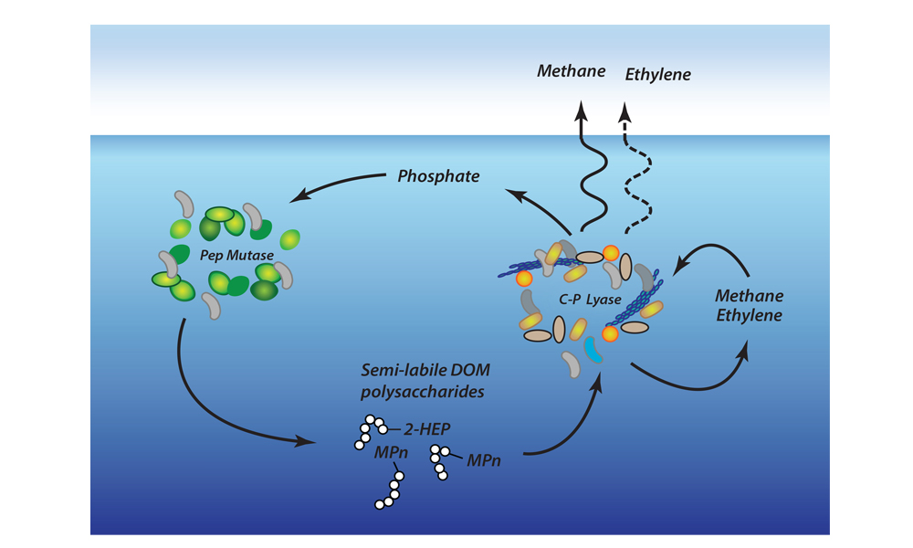
A large fraction of the ocean-to-atmosphere flux of methane occurs in well-oxygenated, open ocean oligotrophic gyres, a phenomenon seemingly at odds with well-known pathways of archaeal methane production under strictly anaerobic conditions. Nearly a decade ago, David Karl and colleagues at the University of Hawaii proposed that water column methane could arise from bacterial metabolism of methylphosphonate, a simple organic compound with reduced phosphorus bonded directly to carbon. However, evidence for this pathway in the environment was lacking. In a recent study published in Nature Geoscience, Repeta et al. (2016) were able to test Karl’s hypothesis using a combination of microbial incubations, genomic analyses, and in-depth chemical analyses of marine dissolved organic matter (DOM). The study revealed that polysaccharides decorated with methyl- and hydroxyethylphosphonate esters are abundant throughout the water column, and that methane and ethylene were quickly produced by natural consortia of bacteria exposed to DOM-amended seawater. Companion knock-out experiments of bacteria isolates further showed that the C-P lyase metabolic pathway was responsible for methane production. Daily cycling of only 0.25% DOM polysaccharide can easily support measured fluxes of marine methane to the atmosphere. Figure from Repeta et al. (2016).

Subtropical Gyre Productivity Sustained by Lateral Nutrient Transport

Posted by mmaheigan 
· Tuesday, December 20th, 2016 

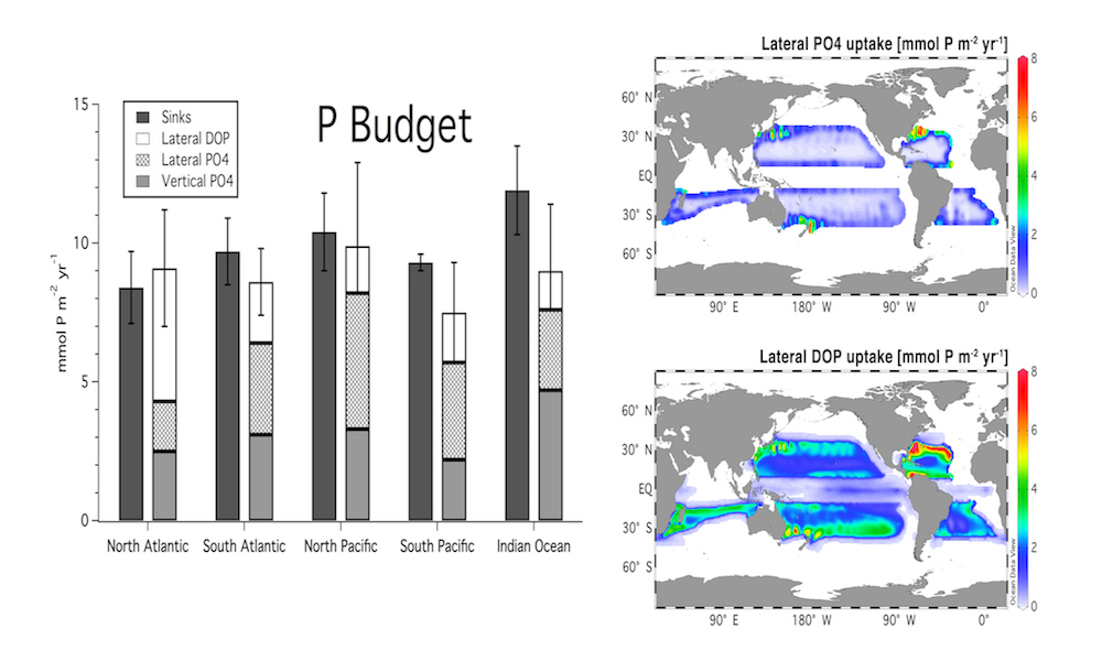
Vertical processes are thought to dominate nutrient resupply across the ocean, however estimated vertical fluxes are insufficient to sustain observed net productivity in the thermally stratified subtropical gyres. A recent study by Letscher et al. (2016) published in Nature Geoscience used a global biogeochemical ocean model to quantify the importance of lateral transport and biological uptake of inorganic and organic forms of nitrogen and phosphorus to the euphotic zone over the low-latitude ocean. Lateral nutrient transport is a major contributor to subtropical nutrient budgets, supplying a third of the nitrogen and up to two-thirds of the phosphorus needed to sustain gyre productivity. Half of the annual lateral nutrient flux occurs during the stratified summer and fall months, helping to explain seasonal patterns of net community production at the time-series sites near Bermuda and Hawaii. Figure from Letscher et al. (2016).

Nutrient Distributions Reveal the Fate of Sinking Particles

Posted by mmaheigan 
· Monday, November 21st, 2016 

The ocean’s “biological pump” regulates the atmosphere-ocean partitioning of carbon dioxide (CO2), and has likely contributed to significant climatic changes over Earth’s history (1, 2). It comprises two processes, separated vertically in the water column: (i) production of organic carbon and export from the surface euphotic zone (0-100m), mostly as sinking particles; and (ii) microbial remineralization of organic carbon to CO2 in deeper waters, where it cannot exchange with the atmosphere.

The depth of particulate organic carbon (POC) remineralization controls the longevity of carbon storage in the ocean (3), and strongly influences the atmospheric CO2 concentration (4). CO2 released in the mesopelagic zone (100-1000m) is returned to the atmosphere on annual to decadal timescales, whereas POC remineralization in the deep ocean (>1000m) sequesters carbon for centuries or longer (5). A common metric for the efficiency of the biological pump is thus the fraction of sinking POC that reaches the deep ocean before remineralization (6), referred to as the particle transfer efficiency, or Teff.

Currently, the factors that govern particle remineralization depth are poorly understood and crudely represented in climate models, compared to the lavish treatment of POC production by autotrophic communities in the surface (7). This compromises our ability to predict the biological pump’s response to anthropogenic warming, and its potential feedback on atmospheric CO2 (8). Over the last decade, a number of studies have identified a promising path towards closing this gap. If systematic spatial variations inTeff can be identified throughout the modern ocean, we might discern their underlying environmental or ecological causes (9, 10). However, direct observations from sediment traps are too sparse to constrain time-mean particle fluxes through the mesopelagic zone at the global scale, and no consensus pattern of Teff has emerged from these analyses.

Particle flux reconstruction

Instead of relying on sparse particle flux observations, a recent study took an alternative approach, leveraging the geochemical signatures that are left behind when particles remineralize (11). Products of remineralization include inorganic nutrients like phosphate (PO43-), whose global distributions are well characterized by hundreds of thousands of shipboard observations (12). In shallow subsurface waters, nutrient accumulation reflects the remineralization of both organic particles and dissolved organic matter, which is advected and entrained from the euphotic zone. Dissolved organic phosphorous (DOP) decomposes rapidly, and is almost completely absent

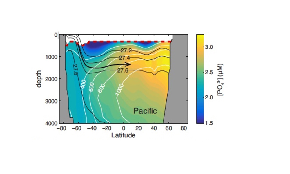
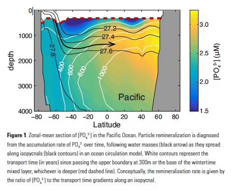
In shallow subsurface waters, nutrient accumulation reflects the remineralization of both organic particles and dissolved organic matter, which is advected and entrained from the euphotic zone. Dissolved organic phosphorous (DOP) decomposes rapidly, and is almost completely absent by depths of ~300m in the stratified low latitude ocean (13), and below the wintertime mixed layer in high latitudes (14). Deeper in the water column, particulate organic phosphorous (POP) remineralization is the only process that generates PO43- within water masses as they flow along isopycnal surfaces (Fig. 1). Rates of POP remineralization can therefore be diagnosed from the accumulation rate of PO43- along transport pathways in an ocean circulation model. This calculation requires a very faithful representation of the large-scale circulation, as provided by the Ocean Circulation Inverse Model (OCIM), whose flow fields are optimized to match observed water mass tracer distributions (15).

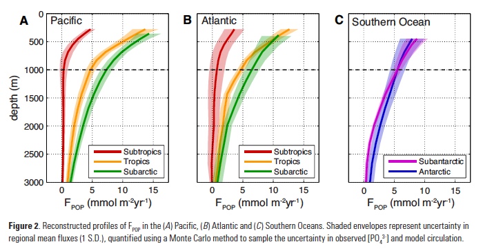
Assuming that organic matter burial in sediments is negligible, the integrated POP remineralization beneath a given depth horizon is equal to the flux of POP (FPOP) through that horizon, allowing complete reconstruction of flux profiles from ~300m to the deep ocean. Averaging these fluxes over large ocean regions serves to extract the large-scale signal from small-scale noise (Fig. 2). Regional-mean FPOP profiles show striking differences in shape and magnitude between subarctic, tropical, and subtropical regions, which are remarkably consistent between the Pacific and Atlantic Oceans (Fig 2a,b). FPOP near 300m is similar in subarctic and tropical zones, but attenuates faster through the mesopelagic in the tropics, reaching values of ~5mmol m-2yr-1 at 1000m, compared to ~7mmol m-2yr-1 in subarctic oceans. Subtropical FPOP attenuates even faster, and is indistinguishable from zero throughout most of the water column. In the Southern Ocean, FPOP is ~5mmol m-2yr-1 at 1000m in both the Antarctic and subantarctic regions, but the subantarctic flux profile attenuates slightly faster (Fig. 2c).

Patterns of transfer efficiency and underlying mechanisms

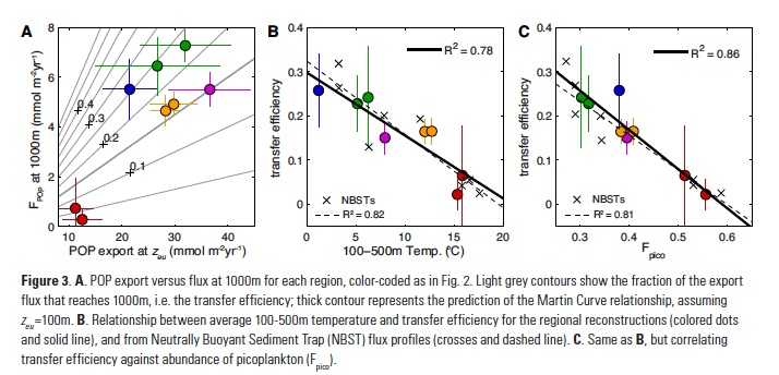
While these reconstructions place a robust constraint on POP fluxes to the deep ocean, they do not constrain rates of POP export at the base of the euphotic zone (zeu) that are needed to estimate the particle transfer efficiency (Teff). Remote sensing approaches are widely used to estimate large-scale organic carbon export, which can be converted to POP using an empirical relationship for particulate P:C ratios (16). However, multiple algorithms have been proposed to estimate net primary production and convert it to export, yielding widely different regional-mean rates (11). One way to pare down this variability is to weight each algorithm based on its ability to reproduce tracer-based export estimates in each ocean region (17, 18). This yields an “ensemble” estimate for the areal-mean POP export rate in each region, and an uncertainty range that reflects both observational error and the variability between satellite algorithms (Fig. 3a).

Combining the ensemble estimates of POP export with reconstructed FPOP at 1000m reveals a systematic pattern of transfer efficiency from zeu to the deep ocean (Fig. 3a).  The subtropics exhibit the lowest Teff of ~5%, significantly lower than expected from the canonical Martin Curve relationship (19), which is often considered to represent an “average” particle flux profile. In the tropics and the subantarctic zone of the Southern Ocean, Teff clusters close to the Martin Curve prediction of ~15%. The subarctic and Antarctic regions (i.e. high latitudes) are the most efficient at delivering the surface export flux to depth with Teff>25%, although these values are also associated with the largest uncertainty (Fig. 3a).

What controls the strong latitudinal variation of transfer efficiency? Particle flux attenuation is determined by the sinking speed and bacterial decomposition rate of particles: fast sinking and slow decomposition both result in greater delivery of organic matter to the deep ocean. Decomposition rates increase as a function of temperature in laboratory incubation studies (20), controlled by the temperature-dependence of bacterial metabolism. In a recent compilation of Neutrally Buoyant Sediment Trap (NBST) observations, particle flux attenuation was strongly correlated with upper ocean temperature between 100-500m (21), consistent with this effect. An almost identical temperature relationship explains ~80% of the variance in reconstructed regional Teff estimates (Fig. 3b).

An equally compelling argument can be made for particle sinking speeds controlling the pattern of Teff. According to the current paradigm of marine food webs (22), communities dominated by small phytoplankton export small particles that sink slowly, relative to the large aggregates and fecal pellets produced when large plankton dominate. The fraction of photosynthetic biomass contributed by tiny picoplankton (Fpico) varies from <30% in subarctic regions to >55% in oligotrophic subtropical regions (23), and explains ~86% of the variance in reconstructed Teff (Fig. 3c). Fpico also predicts flux attenuation in NBST profiles as skillfully as upper-ocean temperature (R2 = 0.81 and 0.82 respectively), but was not considered previously (21). Due to the spatial covariation of these factors in the ocean, statistical analysis alone is insufficient to determine the relative contributions of temperature and particle size to latitudinal variations in transfer efficiency.

Conclusions and future directions

Reconstructing deep-ocean particle fluxes has left us with a clearer understanding of the biological pump in the contemporary ocean and its climate sensitivity. Deep remineralization in high latitude regions results in efficient long-term carbon storage, whereas carbon exported in subtropical regions is recirculated to the atmosphere on short timescales (11). Atmospheric CO2 is likely more sensitive to increased high latitude nutrient utilization during glacial periods than previously recognized, whereas the expansion of subtropical gyres in a warming climate might result in a less efficient biological pump.

One caveat is that the new results highlighted here constrain POP transfer efficiency, not POC, and the two might be decoupled by preferential decomposition of one element relative to the other. The close agreement of these results with Neutrally Buoyant Sediment Trap observations (which measure POC) is encouraging, and suggests that the reconstructed pattern ofTeff is applicable to carbon. More widespread deployment of NBSTs, which circumvent the sampling biases of older sediment trap systems (24), would help confirm or refute this conclusion. A second limitation is that the wide degree of uncertainty in high latitude export rates (Fig. 3a) obscures estimates ofTeff in these regions. New tracer-based methods to integrate export across the seasonal cycle (25) will hopefully close this gap and enable more careful groundtruthing of satellite predictions.

Two plausible mechanisms –particle size and temperature – have been identified to explain large latitudinal variations in transfer efficiency, and new observational systems hold the potential to disentangle their effects. Underwater Visual Profilers (UVP) can now accurately resolve the size distribution of particles in mesopelagic waters (26). Although UVPs provide only instantaneous snapshots (quite literally) of the particle spectrum rather than time-mean properties, large compilations of these data will help establish the spatial pattern of particle size and its relationship to microbial community structure. In parallel, ongoing development of the RESPIRE particle incubator will allow for in-situ measurement of POC respiration (27), and better establish its temperature sensitivity.

Over the next few years, the upcoming EXport Processes in the Ocean from RemoTe Sensing (EXPORTS) campaign stands to revolutionize our understanding of the fate of organic carbon (28). These insights will allow for a more balanced treatment of the “dark side” of the biological pump in global climate models, compared to euphotic zone processes, improving our predictions of biological carbon sequestration in a warming ocean.

Author

By Thomas Weber (University of Rochester)

Acknowledgment

This work was supported by NSF grant OCE-1635414 and the Gordon and Betty Moore Foundation (GBMF 3775).

References

1. J. L. Sarmiento et al., Philos. Trans. R. Soc. A Math. Phys. Eng. Sci. 325, 3–21 (1988).
2. A. Mart.nez-Garc.a et al., Science 343, 1347–50 (2014).
3. U. Passow, C. Carlson, Mar. Ecol. Prog. Ser. 470, 249–271 (2012).
4. E. Y. Kwon, F. Primeau, J. L. Sarmiento, Nat. Geosci. 2, 630–635 (2009).
5. T. Devries, F. Primeau, C. Deutsch, Geophys. Res. Lett. 39, 1–5 (2012).
6. P. J. Lam, S. C. Doney, J. K. B. Bishop, Glob. Biogeochem. Cycles. 25, 1–14 (2011).
7. J. K. Moore, S. C. Doney, J. a. Kleypas, D. M. Glover, I. Y. Fung, Deep. Res. Part II Top. Stud. Oceanogr. 49, 403–462 (2002).
8. L. Bopp et al., Biogeosci. 10, 6225–6245 (2013).
9. S. a. Henson, R. Sanders, E. Madsen, Glob. Biogeochem. Cycles. 26, 1–14 (2012).
10. M. J. Lutz, K. Caldeira, R. B. Dunbar, M. J. Behrenfeld, J. Geophys. Res. 112, C10011 (2007).
11. T. Weber, J. A. Cram, S. W. Leung, T. Devries, C. Deutsch, Proc. Nat. Acad. Sci. 113, 8606–8611 (2016).
12. H. E. Garcia et al., NOAA World Ocean Atlas (2010).
13. J. Abell, S. Emerson, P. Renaud, J. Mar. Res. 58, 203–222 (2000).
14. S. Torres-Vald.s et al., Glob. Biogeochem. Cycles. 23, 1–16 (2009).
15. T. Devries, Glob. Biogeochem. Cycles. 28, 631–647 (2014).
16. E. D. Galbraith, A. C. Martiny, Proc. Nat. Acad. Sci., 201423917 (2015).
17. M. K. Reuer, B. A. Barnett, M. L. Bender, P. G. Falkowski, M. B. Hendricks, Deep. Res. Part I Oceanogr. Res. Pap. 54, 951–974 (2007).
18. S. Emerson, Glob. Biogeochem. Cycles. 28, 14–28 (2014).
19. J. H. Martin, G. A. Knauer, D. M. Karl, W. W. Broenkow, Deep Sea Res. Part A, Oceanogr. Res. Pap. 34, 267–285 (1987).
20. M. H. Iversen, H. Ploug, Biogeosciences. 10, 4073–4085 (2013).
21. C. M. Marsay, R. J. Sanders, S. A. Henson, K. Pabortsava, E. P. Achterberg, Proc. Nat. Acad. Sci., 112, 1089–1094 (2014).
22. D. A. Siegel et al., Glob. Biogeochem. Cycles. 28, 181–196 (2014).
23. T. Hirata et al., Biogeosci. 8, 311–327 (2011).
24. K. O. Buesseler et al., Science 316, 567–570 (2007).
25. S. M. Bushinsky, S. Emerson, Glob. Biogeochem. Cycles. 29, 2050–2060 (2015).
26. M. Picheral et al., Limnol. Oceanogr. Methods. 8, 462–473 (2010).
27. A. M. P. McDonnell, P. W. Boyd, K. O. Buesseler, Glob. Biogeochem. Cycles. 29, 175–193 (2015).
28. D. A. Siegel et al., Front. Mar. Sci. 3, 1–10 (2016).

Marine mixotrophs exploit multiple resource pools to balance supply and demand

Posted by mmaheigan 
· Sunday, November 20th, 2016 

“So, in the sea, there are certain objects concerning which one would be at a loss to determine whether they be animal or vegetable.”  Aristotle, The History of Animals

Our understanding of marine ecosystems is strongly influenced by the terrestrial macroscopic world we see around us. For example, the distinction between phytoplankton and zooplankton reflects the very familiar divide between plants and animals. Mixotrophs are organisms that blur this distinction by combining photosynthetic carbon fixation and the uptake of inorganic nutrients with the ingestion of living prey (1). In the macroscopic terrestrial realm, the obvious examples of mixotrophs are the carnivorous plants. These organisms are so well known because they confound the otherwise clear divide between autotrophic plants and heterotrophic animals – in terrestrial environments, mixotrophs are the exception rather than the rule. There appear to be numerous reasons for this dichotomy involving constraints on surface area to volume ratios, the energetic demands of predation, and access to essential nutrients and water. Without dwelling on these aspects of macroscopic terrestrial ecology, it appears that many of the most important constraints are relaxed in aquatic microbial communities. Plankton have no need for the fixed root structures that would prevent motility, and in the three-dimensional fluid environment, they are readily exposed to both inorganic nutrients and prey. In addition, their small size and high surface area to volume ratios increase the potential efficiency of light capture and nutrient uptake. As such, mixotrophy is a common and widely recognised phenomenon in marine ecosystems. It has been identified in a very broad range of planktonic taxa and is found throughout the eukaryotic tree of life. Despite its known prevalence, the potential impacts of mixotrophy on the global cycling of nutrients and carbon are far from clear. In this article, I discuss the ecological niche and biogeochemical role of mixotrophs in marine microbial communities, describing some recent advances and identifying future challenges.

A ubiquitous and important strategy

Mixotrophy appears to be a very broadly distributed trait, appearing in all marine biomes from the shelf seas (2) to the oligotrophic gyres (3), and from the tropics (4) to the polar oceans (5). Within these environments, mixotrophy is often a highly successful strategy. For example, in the subtropical Atlantic, mixotrophic plankton make up >80% of the pigmented biomass, and are also responsible for 40-95% of grazing on bacteria (3, 4). Similar abundances and impacts have also been observed in coastal regions (2, 6).

How does the observed prevalence of mixotrophy affect the biogeochemical and ecological function of marine communities? To understand the potential answers to this question, it is helpful to review the constraints associated with the assumption of a strict dichotomy between autotrophic phytoplankton and heterotrophic zooplankton. Within this paradigm, primary production is restricted to the base of the food web, tightly coupled to the supply of limiting nutrients. Furthermore, the vertical export of
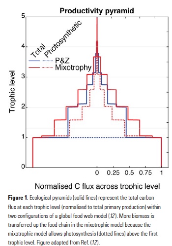
carbon is limited by the supply of exogenous (or “new”) nutrients (7), since any local regeneration of nutrients from organic matter is also associated with the local remineralisation of dissolved inorganic carbon. Energy and biomass are passed up the food web, but the transfer across trophic levels is highly inefficient (8) (Fig. 1) because the energetic demands of strictly heterotrophic consumers can only be met by catabolic respiration.

In the mixotrophic paradigm, several of these constraints are relaxed. Primary production is no longer exclusively dependent on the supply of inorganic nutrients because mixotrophs can support photosynthesis with nutrients derived from their prey. This mechanism takes advantage of the size-structured nature of marine communities (9), with larger organisms avoiding competitive exclusion by eating their smaller and more efficient competitors (10-12). In addition, the energetic demands of mixotrophic consumers can be offset by phototrophy, leading to increased efficiency of carbon transfer through the food web (Fig. 1). These two mechanisms dictate that mixotrophic ecosystems can fix and export more carbon for the same supply of limiting nutrient, relative to an ecosystem strictly divided between autotrophic phytoplankton and heterotrophic zooplankton (12).

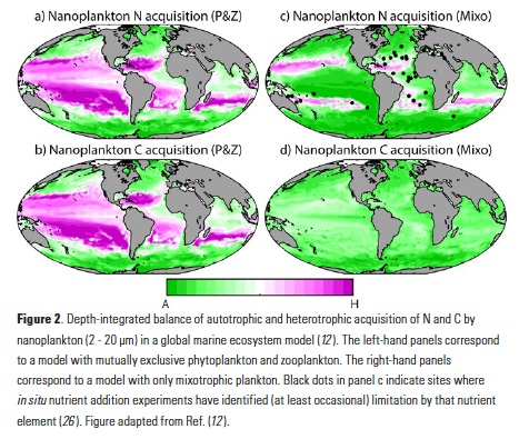
The trophic flexibility associated with mixotrophy appears likely to have a profound effect on marine ecosystem function at the global scale. Fig. 2 contrasts the simulated fluxes of carbon and nitrogen through the intermediate nanoplankton (2-20 μm diameter) size class of a global ecosystem model (12). The left-hand maps show the balance of autotrophic and heterotrophic resource acquisition in a model with mutually exclusive phytoplankton and zooplankton. At low latitudes and especially in the
oligotrophic subtropical gyres, the inorganic nitrogen supply is acquired almost exclusively by the smallest and most competitive phytoplankton (not shown). This leaves an inadequate supply for larger and less competitive phytoplankton, and as such, the larger size classes are dominated by zooplankton (as indicated by the purple shading in Fig. 2a, b). In the more productive polar oceans and upwelling zones, grazing pressure prevents the smaller phytoplankton from exhausting the inorganic nitrogen supply, leaving enough for the larger phytoplankton to thrive in these regions (as indicated by the green shading).

The right-hand maps in Fig. 2 show the balance of autotrophic and heterotrophic resource acquisition in the intermediate size-class of an otherwise identical model containing only mixotrophic plankton. As in the model with mutually exclusive phytoplankton and zooplankton, the inorganic nitrogen supply in the oligotrophic gyres is exhausted by the smallest phytoplankton (see the purple shading in Fig. 2c). However, Fig. 2d indicates that this is not enough to stop photosynthetic carbon fixation among the mixotrophic nanoplankton. The nitrogen acquired from prey is enough to support considerable photosynthesis in a size class for which phototrophy would otherwise be impossible. For the same supply of inorganic nutrients, this additional supply of organic carbon serves to enhance the transfer of energy and biomass through the microbial food web, increasing community carbon:nutrient ratios and leading to as much as a three-fold increase in mean organism size and a 35% increase in vertical carbon flux (12).

Trophic diversity and ecosystem function

Marine mixotrophs are broadly distributed across the eukaryotic tree of life (13). The ability to combine photosynthesis with the digestion of prey has been identified in ciliates, cryptophytes, dinoflagellates, foraminifera, radiolarians, and coccolithophores (14). Perhaps the only major group with no identified examples of mixotrophy are the diatoms, which have silica cell walls that may hinder ingestion of prey. While some mixotroph species are conceptually more like plants (that eat), others are more like animals (that photosynthesise). A number of conceptual models have been developed to account for this observed diversity. One scheme (15) identified three primarily autotrophic groups that use prey for carbon, nitrogen or trace compounds, and two primarily heterotrophic groups that use photosynthesis to delay starvation or to increase metabolic efficiency. More recently, an alternative classification (16, 17) identified three key groups on a spectrum between strict phototrophy and strict phagotrophy. According to this classification, primarily autotrophic mixotrophs can synthesise and fully regulate their own chloroplasts, whereas more heterotrophic forms must rely on chloroplasts stolen from their prey. Among this latter group, the more specialised species exploit only a limited number of prey species, but can manage and retain stolen chloroplasts for relatively long periods. In contrast, generalist mixotrophs target a much wider range of prey, but any stolen chloroplasts will degrade within a matter of hours or days (18).

This diversity of trophic strategies is clearly more than most biogeochemical modellers would be prepared to incorporate into their global models. Nonetheless, many of the conceptual groups identified above are associated with the ability of mixotrophs to rectify the often-imbalanced supply of essential resources in marine ecosystems (19). This is clearly relevant to the coupling of elemental cycles in the ocean, and it appears likely that the relative abundance of different trophic strategies can impact the biogeochemical function of marine communities (1, 20). For example, recent work suggests that a differential temperature sensitivity of autotrophic and heterotrophic processes can push mixotrophic species towards a more heterotrophic metabolism with increasing temperatures (21). An important goal is therefore to accurately quantify and account for the global-scale effects of mixotrophy on the transfer of energy and biomass through the marine food web and the export of carbon into the deep ocean. We also need to assess how these effects might be sensitive to changing environmental conditions in the past, present, and future.

These processes are not resolved in most contemporary models of the marine ecosystem, which are often based on the representation of a limited number of discrete plankton functional types (22). In terms of resolving mixotrophy, it is not the case that these models have overlooked the one mixotrophic group. Instead, it may be more accurate to say that the groups already included have been falsely divided between two artificially distinct categories. As such, modelling mixotrophy in marine ecosystems is not just a case of increasing complexity by adding an additional mixotrophic component. Instead, progress can be made by understanding the position, connectivity, and influence of mixotrophic and non-mixotrophic organisms within the food web as an emergent property of their environment, ecology, and known eco-physiological traits. This is not a simple task, but progress might be made by identifying the fundamental traits that underpin the observed diversity of functional groups. To this end, a recurring theme in mixotroph ecology is that plankton exist on a spectrum between strict autotrophy and strict heterotrophy (14, 23, 24). Competition along this spectrum is typically framed in terms of the costs and benefits of different modes of nutrition. Accurate quantification of these costs and benefits should allow for a much clearer understanding of the trade-offs between different mixotrophic strategies (25), and how they are selected in different environments. In the future, a combination of culture experiments, targeted field studies, and mathematical models should help to achieve this goal, such that this important ecological mechanism can be reliably and parsimoniously incorporated into global models of marine ecosystem function.

Author

Ben Ward (University of Bristol)

References

1. Stoecker, D. K., Hansen, P. J., Caron, D. A. & Mitra, Annual Rev. Marine Sci. 9, forthcoming (2017).
2. Unrein, F., Gasol, J. M., Not, F., Forn, I. & Massana, R. The ISME Journal 8, 164–176 (2013).
3. Zubkov, M. V. & Tarran, G. A. Nature 455, 224–227 (2008).
4. Hartmann, M. et al. Proc. Nat. Acad. Sci. 5756–5760 (2012). doi:10.1073/pnas.1118179109
5. Gast, R. J. et al. J. Phycol. 42, 233–242 (2006).
6. Havskum, H. & Riemann, B. Marine Ecol. Prog. Ser. 137, 251–263 (1996).
7. Dugdale, R. C. & Goering, J. J. Limnol. Oceanogr. 12, 196–206 (1967).
8. Lindeman, R. L. Ecol. 23, 399–417 (1942).
9. Sieburth, J. M., Smetacek, V. & Lenz, J. Limnol. Oceanogr. 23, 1256–1263 (1978).
10. hingstad, T. F., Havskum, H., Garde, K. & Riemann, B. Ecol. 77, 2108–2118 (1996).
11. Våge, S., Castellani, M., Giske, J. & Thingstad, T. F. Aquatic Ecol. 47, 329–347 (2013).
12. Ward, B. A. & Follows, M. J. Proc. Nat. Acad. Sci. 113, 2958–2963 (2016).

A chalkier ocean? Multi-decadal increases in North Atlantic coccolithophore populations

Posted by mmaheigan 
· Saturday, November 19th, 2016 

Coccolithophores and the carbon cycle

Increasing atmospheric CO2 concentrations are resulting in both warmer sea surface temperatures due to the greenhouse effect and increasingly carbon-rich surface waters. The ocean has absorbed roughly one third of anthropogenic carbon emissions (1), causing a shift in carbon chemistry equilibrium to more acidic conditions with lower calcium carbonate saturation states (ocean acidification). Organisms that produce calcium carbonate structures are thought to be particularly susceptible to these changes (2-4).

Coccolithophores are the most abundant type of calcifying unicellular micro-algae in the ocean, producing microscopic calcium carbonate plates called coccoliths (5). Low-pH conditions have been shown to disrupt the formation of coccoliths (calcification; e.g., (6)). Therefore, it is generally expected that a higher-CO2 ocean will cause a reduction in calcification rates or a decrease in the abundance of these calcifiers. Such changes could have far-reaching consequences for marine ecosystems, as well as global carbon cycling and carbon export to the deep sea.

Coccolithophores use sunlight to synthesize both organic carbon through photosynthesis and particulate inorganic carbon (PIC) through calcification. Detrital coccolithophore shells form aggregates with organic material, enhancing carbon export to the deep sea (7). Coccolithophores also produce dimethyl sulfide (DMS), a climatically relevant trace gas that impacts cloud formation, ultimately influencing Earth’s albedo (8, 9). At the ecosystem level, coccolithophores compete for nutrients with other phytoplankton and provide energy for the rest of the marine food web. Coccolithophores have a broad range of irradiance, temperature, and salinity tolerances (10, 11). Moreover, their relatively low nutrient requirements and slow growth rates offer a competitive advantage under projected global warming and ocean stratification (5). This plasticity and opportunistic behavior can be critical for persistence in a changing oceanic environment. Given the wide range of biogeochemical and ecological processes impacted by coccolithophores, it is important to assess how anthropogenic changes may affect coccolithophore growth and calcification.

Many laboratory studies have investigated the impact of future environmental conditions on coccolithophores by decreasing pH, increasing dissolved inorganic carbon, and increasing temperature to mimic end-of-century projections. However, these have often yielded conflicting results: Some show a decrease, while others show no change or even increased calcification (e.g., (6, 12, 13)). For example, laboratory simulations of contemporary oceanic changes (increasing CO2 and decreasing pH) show that coccolithophores have the ability to modulate organic carbon production and calcification in response to variable amounts of dissolved inorganic carbon (DIC) but that low pH only affects these processes below a certain threshold (14). Another study indicated that coccolithophores could adapt to warming and highCO2 levels over the course of a year, maintaining their relative particulate organic carbon (POC) and PIC production per cell (15). One of the limitations of all laboratory experiments is that only a handful of species (and strains) are studied, which is only a tiny fraction of the diversity present in the oceans. Given the challenges of extrapolating laboratory results to real world oceans, studying recent trends in natural populations may lead to important insights.

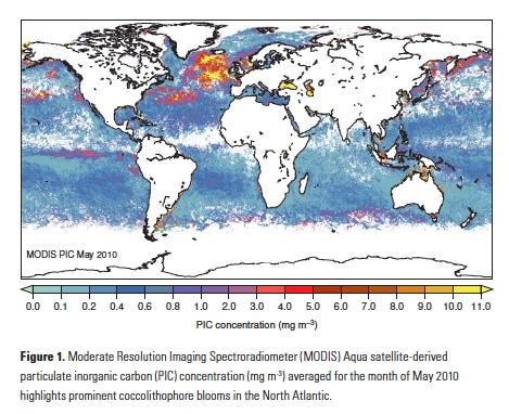
The North Atlantic is both a region with rapid accumulation of anthropogenic CO2 (1) and an important coccolithophore habitat (Fig. 1), making this region a good starting point to search for in situ evidence of anthropogenic carbon effects on diverse coccolithophore populations. Two recent studies did precisely that: Rivero- Calle et al. (2015)(16) in the subpolar North Atlantic, and Krumhardt et al. (2016)(17) in the North Atlantic subtropical gyre. Using independent datasets, these two studies concluded that coccolithophores in the North Atlantic appear to be increasing in abundance and, contrary to the prevailing paradigm, responding positively to the extra carbon in the upper mixed layer.

Evidence from long-term in situ monitoring (two independent case studies)

Rivero-Calle et al. (2015) used data from the Continuous Plankton Recorder (CPR), a filtering device installed on ships of opportunity, to assess changes in coccolithophore populations from 1965 to 2010 in the subpolar North Atlantic. This highly productive, temperate region is dominated by large phytoplankton and characterized by strong seasonal changes in the mixed layer depth, nutrient upwelling, and gas exchange that lead to intense, well-established spring phytoplankton blooms.

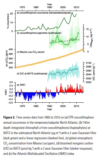
Because coccolithophore cells are smaller than the mesh size used by the CPR, they cannot be accurately quantified in the CPR data set. Some coccolithophore cells do, however, get caught in the mesh and their occurrence (i.e. probability of presence) can be calculated and serve as a proxy for coccolithophore abundance. Using recorded presence or absence of coccolithophores over this multidecadal time-series, the authors showed that coccolithophore occurrence in the subpolar North Atlantic increased from being present in only 1% of samples to > 20% over the past five decades (Fig. 2). To assess the importance of a wide range of diverse environmental drivers on changes in coccolithophore occurrence, Rivero-Calle and co-authors used random forest statistical models. Specifically, they examined more than 20 possible biological and physical predictors, including CO2 concentrations, nutrients, sea surface temperature and the Atlantic Multidecadal Oscillation (AMO), as well as possible predators and competitors. Global and local CO2 concentrations were shown to be the best predictors of coccolithophore occurrence. The AMO, which has been in a positive phase since the mid-1990s (Fig. 2) and is associated with anomalously warmer temperatures over the North Atlantic, was also a good predictor of coccolithophore occurrence, but not as strong of a predictor as CO2.

The authors hypothesize that the synergistic effects of increasing anthropogenic CO2, the recent positive phase of the AMO, and increasing global temperatures contributed to the observed increase in coccolithophore occurrence in the CPR samples from 1965 to 2010. Complementing the Rivero-Calle et al. (2015) study, Krumhardt et al. (2016) used phytoplankton pigment concentration data from the long-running Bermuda Atlantic Time-series Study (BATS) and satellite-derived PIC data to assess recent changes in coccolithophore abundance in the subtropical North Atlantic. This region of the North Atlantic is characterized by Ekman convergence and downwelling, resulting in an oligotrophic environment. Despite relatively low productivity, subtropical gyres cover vast expanses of the global ocean and are thus important on a global scale.

In the North Atlantic subtropical gyre, researchers at BATS have performed phytoplankton pigment analyses since the late 1980s, as well as a suite of other oceanographic measurements (nutrients, temperature, salinity, etc.). This rich dataset provided insight into phytoplankton dynamics occurring at BATS over the past two decades. Coccolithophores contain a suite of pigments distinctive to haptophytes. Though there are many species of non-calcifying haptophytes in the ocean (18), the main contributors to the haptophyte community in oligotrophic gyres are coccolithophores (19). Using a constant haptophyte pigment to chlorophyll a ratio Krumhardt et al. (2016) quantified relative abundance of the coccolithophore chlorophyll a (Chlahapto) over the BATS time-series. A simple linear regression revealed that coccolithophore pigments have increased in the upper euphotic zone by 37% from 1990 to 2012 (Figure 2). On the other hand, total chlorophyll a at BATS only increased slightly over this time period.

While satellite-derived chlorophyll a is used as a proxy for biomass and abundance of the entire phytoplankton community (20), satellite-derived PIC is formulated to specifically retrieve calcium carbonate from coccolithophore shells (21, 22). Therefore, satellite PIC can be used as a proxy for coccolithophore abundance. Although there has been virtually no change in total chlorophyll a over most of the North Atlantic subtropical gyre over the satellite era (1998-2014), predominantly positive trends were shown over this time period for PIC (17). This indicates that coccolithophore populations appear to be increasing over and above other phytoplankton species in the subtropical gyre.

Like Rivero-Calle et al., Krumhardt et al. explored possible environmental drivers of this increase in coccolithophore pigments at BATS and coccolithophore PIC throughout the gyre. They performed linear correlations between variability of hypothesized drivers and coccolithophore chlorophyll a concentrations at the BATS site. Increasing DIC, specifically the bicarbonate ion (HCO3–) fraction, showed a strong positive correlation with pigments from coccolithophores, explaining a significant fraction of the coccolithophore pigment variability. DIC in the upper mixed layer at BATS has been increasing steadily over the past several decades from absorption of anthropogenic CO2 (Fig. 2; 23) and coccolithophores may be responding to this. But how does extra carbon in the water explain the increases in coccolithophore populations?

Environmental controls on coccolithophore growth

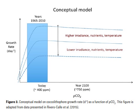
A few studies have shown that, in contrast to most other phytoplankton, coccolithophore photosynthesis (specifically, the widespread coccolithophore species Emiliania huxleyi) can be carbon-limited at today’s CO2 levels (e.g., 14, 24). This suggests that increases in surface DIC (e.g., due to the uptake of anthropogenic CO2) may alleviate growth limitation of coccolithophores. By reducing the amount of energy spent on carbon concentrating mechanisms, coccolithophores may invest in other metabolic processes such as growth, PIC or POC production. This explains why a relatively small increase in DIC could increase coccolithophore competitive ability, especially in oligotrophic environments where phytoplankton are routinely in competition for scarce nutrients. Rivero-Calle and co-authors compiled numerous published laboratory studies that assessed coccolithophore growth rates as a function of pCO2. The compilation, which included several species and strains of coccolithophores, showed that there is a quasi-hyperbolic increase in coccolithophore growth rates as pCO2 increases (Fig. 3). The range of local pCO2 concentrations in the subpolar/temperate North Atlantic from 1965 to 2010 (~175 to 435 ppm) spanned the pCO2 levels over which there is a substantial increase in published coccolithophore growth rates (Fig. 3). Growth rates tend to stabilize at ~500 ppmCO2, indicating that coccolithophore populations may continue to respond positively to increasing CO2 for the next few decades.

Other environmental factors (e.g., temperature, light, and available nutrients) may also impact and modulate coccolithophore growth rates, resulting in a net neutral or net negative impact in spite of increasing atmospheric (marine) CO2 (DIC) concentrations (see conceptual model, Fig. 3). For example, severe nutrient limitation in the subtropics may cause coccolithophores to be outcompeted by smaller marine cyanobacteria. In the subpolar North Atlantic, nutrients are more plentiful than in the subtropics, but Earth system models have predicted that climatic warming in this region may result in increased water column stratification (25). Under these stratified low-nutrient conditions, smaller phytoplankton such as coccolithophores could become more prevalent at the expense of larger phytoplankton such as diatoms (26, 27). However, if nutrient concentrations decline to the point at which they become the limiting factor for growth, then coccolithophore populations will also be negatively affected. Furthermore, the associated drop in pH from CO2 dissolving into the upper mixed layer can eventually be detrimental to coccolithophore growth and calcification. Specifically, pH values below 7.7 negatively affected the coccolithophore Emiliania huxleyi in laboratory experiments (14), though most oceanic regions will not show such a low pH any time in the near future. In short, anthropogenic CO2 entering the ocean may allow coccolithophores a competitive edge in the near future in some regions such as the North Atlantic, but other compounding influences from anthropogenic climate change such as severe nutrient limitation or ocean acidification are also important to consider, particularly in the oligotrophic gyres.

Open questions and future directions

While recent work has provided new insight into the impact of several environmental factors (irradiance, nutrients, temperature, pH, DIC) on coccolithophores, many questions remain. Among these, the vertical distribution of coccolithophore communities, grazing rates, and viral infection on coccolithophores, and species-specific responses to environmental change are relatively unexplored areas of research. For instance, some studies have shown species-specific and even strain-specific variability in the response of coccolithophores to CO2 (28, 29), but how various coccolithophore species respond to nutrient or light limitation is relatively unknown. Due to its cosmopolitan distribution and ability to grow relatively easily in the lab, E. huxleyi, has become the “lab rat” species. However, it may not be the most important calcite producer globally (30), nor the most representative of the coccolithophore group as a whole. As part of its peculiarities, E. huxleyi can both produce several layers of coccoliths and also exhibit a naked form without coccoliths, posing questions about the importance of non-calcified forms in the projected acidified oceans and about the role of calcification per se (31). Indeed, the fundamental question of why coccolithophores calcify is still unresolved and may vary between species (5, 32). In addition, while we recognize that some zooplankton groups graze on coccolithophores (coccoliths have been found in pelagic tintinnid ciliates (33), as well as copepod guts and fecal pellets (34-36)), little is known about predation rates or specificity in natural populations. Finally, we know that viruses can also cause bloom termination and that E. huxleyi can induce coccolith detachment to avoid viral invasion (37); however, there are still many unknowns related to bloom dynamics. Until we understand what drives coccolithophore calcification and variations in growth and mortality rates, we will have an incomplete picture of the role that coccolithophores play in marine ecology and the carbon cycle.

Krumhardt et al (2016) and Rivero-Calle et al (2016) both arrive at a simple conclusion: Coccolithophore presence in the North Atlantic is increasing. The common denominators in this equation are increasing global CO2 levels and increasing global surface temperatures. Therefore, even given regional oceanic variability in environmental drivers, we might expect to see similar trends in coccolithophore abundance in other regions. Given coccolithophores’ positive response to increasing anthropogenic CO2 and temperature, as well as general fitness under conditions that may be more prevalent in the future ocean, coccolithophores may become an even bigger player in the marine carbon cycle, which may have unexpected consequences.

Authors
Kristen Krumhardt (University of Colorado Boulder)
Sara Rivero-Calle (University of Southern California, Los Angeles)
Acknowledgments
We would like to thank co-authors on the Rivero-Calle et al. (2015) and Krumhardt et al. (2016) studies for their contributions to the research described. We also would like to thank Nikki Lovenduski and Naomi Levine for helpful comments in composing this OCB Newsletter piece. Many thanks to APL, NSF, NOAA and NASA for funding, and SAHFOS, ICOADS, the BATS research group, and NASA for their long-term data and making it freely available.

References

1. C. L. Sabine et al., Science 305 (2004).
2. Feely et al., Science 305, 362-366 (2004).
3. J. C. Orr et al., Nature 437, 681-686 (2005).
4. K. J. Kroeker et al., Global Change Biology 19, 1884-1896 (2013).
5. B. Rost, U. Riebesell, In Coccolithophores: from Molecular Processes to Global Impact, 99-125 (2004).
6. U. Riebesell et al., Nature 407, 364-367 (2000).
7. C. Klaas, D. E. Archer, Glob.Biogeochem. Cycles 16, (2002).
8. M. D. Keller, W. K. Bellows, R. R. L. Guillard, Acs Symposium Series 393, 167-182 (1989).
9. S. M. Vallina, R. Simo, Science 315, 506-508 (2007).
10. T. Tyrrell, A. Merico, In H. R. Thierstein, J. R. Young, Eds.,Coccolithophores: from Molecular Processes to Global Impact (2004),pp. 75-97.
11. W. M. Balch, In Coccolithophores: from Molecular Processes to Global Impact, 165-190 (2004).
12. M. D. Iglesias-Rodriguez et al., Science 320, 336-340 (2008).
13. S. Sett et al., Plos One 9, (2014).
14. L. T. Bach et al., New Phytol. 199, 121-134 (2013).
15. L. Schluter et al., Nature Clim. Change 4, 1024-1030 (2014).
16. S. Rivero-Calle, A. Gnanadesikan, C. E. Del Castillo, W. M.Balch, S. D. Guikema, Science 350, 1533-1537 (2015).
17. K. M. Krumhardt, N. S. Lovenduski, N. M. Freeman, N. R.Bates, Biogeosci. 13, 1163-1177 (2016).
18. H. Liu et al., Proc. Nat. Acad. Sci. 106, 12803-12808 (2009).
19. Y. Dandonneau, Y. Montel, J. Blanchot, J. Giraudeau, J. Neveux, Deep-Sea Res. Part I-Oceanographic Research Papers 53, 689-712(2006).
20. M. J. Behrenfeld, P. G. Falkowski, Limnol. Oceanogr. 42, 1-20(1997).
21. H. R. Gordon et al. (Geochemical Research Letters, 2001), vol.28, pp. 1587-1590.
22. W. M. Balch, H. R. Gordon, B. C. Bowler, D. T. Drapeau, E. S.
Booth, J. Geophys. Res.Oceans 110 (2005).
23. N. R. Bates et al., Oceanogr. 27, 126-141 (2014).
24. B. Rost, U. Riebesell, S. Burkhardt, D. Sultemeyer, Limnol.Oceanogr. 48, 55-67 (2003).
25. A. Cabr., I. Marinov, S. Leung, Clim.Dyn. 1-28 (2014).
26. L. Bopp, O. Aumont, P. Cadule, S. Alvain, M. Gehlen, Geophys.Res. Lett. 32, (2005).
27. I. Marinov, S. C. Doney, I. D. Lima, Biogeosci. 7, 3941-3959 (2010).
28. Langer et al., Geochem. Geophys. Geosys. 7, (2006).
29. Langer, G. Nehrke, I. Probert, J. Ly, P. Ziveri, Biogeosci. 6, 2637-2646 (2009).
30. C. J. Daniels et al., Marine Ecol. Prog. Ser. 555, 29-47 (2016).
31. M. N. Muller, T. W. Trull, G. M. Hallegraeff, Marine Ecol. Prog.Ser. 531, 81-90 (2015).
32. F. M. Monteiro et al., Science Advances 2, (2016).
33. J. Henjes, P. Assmy, Protist 159, 239-250 (2008).
34. S. Honjo, M. R. Roman, J. Marine Res. 36, 45-57 (1978).
35. R. P. Harris, Marine Biol. 119, 431-439 (1994).
36. J. D. Milliman et al., Deep Sea Res. Part I: Oceanographic Research Papers 46, 1653-1669 (1999).
37. M. Frada, I. Probert, M. J. Allen, W. H. Wilson, C. de Vargas, Proc. Nat. Acad. Sci. 105, 15944-15949 (2008).

What controls the distribution of dissolved organic carbon in the surface ocean?

Posted by mmaheigan 
· Friday, November 11th, 2016 

Around 662 billion tons of organic carbon are dissolved in the ocean, making the pool one of Earth’s major, exchangeable carbon reservoirs. Dissolved organic carbon (DOC) has many ecological functions. It can form complexes with metals (1); absorb UV and visible light, acting as a “sunscreen” for marine microorganisms and controlling primary production in the upper water column (2); it has antioxidant activity, reacting with free radicals in the media (3); but most importantly, it serves as substrate for the microbial loop and as a vehicle for carbon sequestration in the ocean. Therefore, DOC plays an important role in climate on geological time scales.

Because the amount of atmospheric CO2 is of the same magnitude as the DOC pool, and is closely linked to it through exchange, variations in one of these reservoirs can affect the other, impacting the carbon cycle with consequences for climate. Significant net DOC remineralization would lead to an increase of atmospheric CO2, enhancing greenhouse warming at the surface of the Earth. Net oxidation of only 1% of the seawater DOC pool within 1 year would be sufficient to generate a CO2 flux of 7 PgC/yr, comparable to that produced annually by fossil fuel combustion (4). It has also been proposed that a large-scale oxidation of DOC may have prevented a dramatic global glaciation (‘snowball earth’) in the Neoproterozoic period (5).

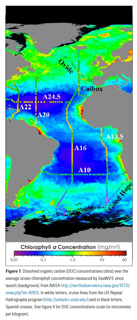
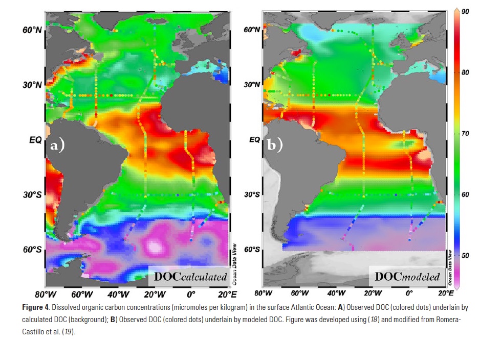
Despite its importance, knowledge about DOC dynamics is relatively limited; in fact, it was considered highly inert until about three decades ago when a new analytical technique for measuring it via high-temperature catalytic oxidation stimulated new interest (6). The technique eventually provided more accurate DOC values, showing that it was more involved in the carbon cycle than previously thought and that its concentrations vary with depth, time, and location. Considering DOC distributions observed in the surface Atlantic Ocean (Fig. 1), we see values in the subtropical gyres of 65-70 µmol Kg-1, the highest concentrations in the tropics (> 70 µmol Kg-1), the lowest in the Southern Ocean (< 50 µmol Kg-1), and moderate concentrations in the northern North Atlantic (55-60 µmol Kg-1); this pattern is consistent in other ocean basins. So what controls this distribution and can we predict it? Even with improved analytical techniques, DOC is not a variable that can be measured easily at sea, and the sampling must be done carefully since it is easy to contaminate. Therefore, DOC data are typically fewer than those of other more readily determined variables such as nutrients and oxygen. If we could predict DOC from variables for which much greater global ocean coverage exists, we could fill the very large spatial and temporal gaps in the DOC fields.

DOC is produced in the upper water column by phytoplankton (primary producers). Actually, half of the inorganic carbon that is fixed by phytoplankton is transformed to DOC. Heterotrophic microbes consume most of that DOC, but ~ 4% of global annual net primary production (~ 2 Pg C y-1) (7) accumulates as DOC, much of which is exported to the mesopelagic via vertical mixing and convergence, thus contributing to the biological carbon pump.

New primary production, the foundation of a system’s net community production (NCP), depends on new nutrients reaching the euphotic zone, which happens primarily via upwelling in divergence zones and winter vertical mixing. NCP is the balance of the carbon generated by primary producers minus that lost through heterotrophic respiration (prokaryotes and animals). It can be estimated either by a loss of reactants (CO2 or nutrients) or a gain in products (suspended POC, DOC, and export production) (8).

In our work, we needed to establish the fraction of NCP that was present in dissolved form (i.e., the net DOC production ratio, or NDPr). For that, we simply estimated NCP from the nitrate (NO3–) that is consumed in the euphotic zone (DNO3–):

ΔNO3– = new NO3– (introduced from deeper layers) – remaining NO3– (at surface) (Eq. 1)

In the same way, we also calculated net accumulated DOC, or ΔDOC:

ΔDOC = DOC in euphotic zone – DOC introduced from deeper layers (Eq. 2)

The ratio between ΔDOC and ΔNO3– gave us the NDPr:

NDPr = ΔDOC/ΔNO3– (Eq. 3)

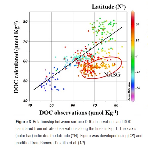
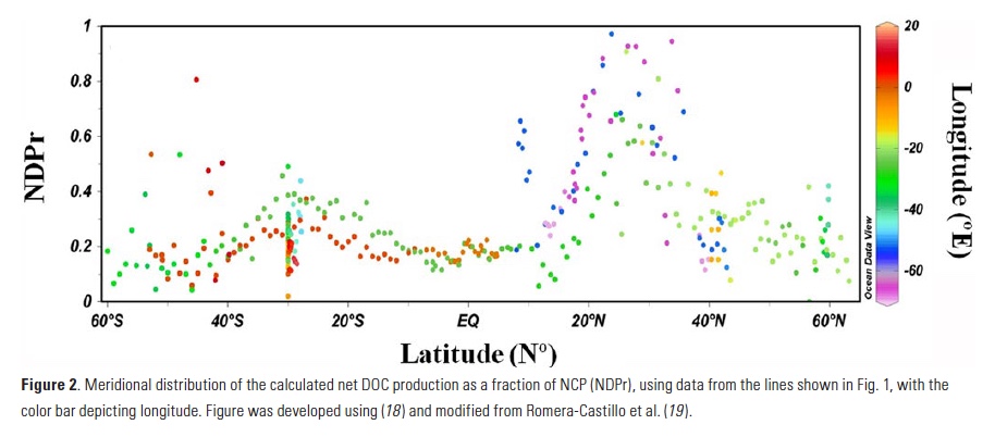
NDPr was calculated throughout the Atlantic Ocean using observations of DOC and NO3– from >15 international oceanographic cruises over the last decade, including those occupied by the US Repeat Hydrography program (Fig. 1). Values of NDPr mostly varied between 0.1 and 0.4 (Fig. 2), with the exception of the North Atlantic Subtropical Gyre (NASG), where NDPr values reach >0.8 at times. After sensitivity testing, we applied a NDPr value of 0.17 to the entire basin, which yielded the smallest error between calculated and observed DOC concentrations. Applying this NDPr value to ΔNO3– (i.e. NCP) obtained from cruise data, we estimate ΔDOC (Eq. 4), in which 6.6 is the molar conversion from N to C units:

ΔDOC= ΔNO3– * 6.6 * 0.17 = NCP * 0.17 (Eq. 4)

To obtain the calculated DOC concentration (DOCcalculated), we added the DOC concentration of underlying source waters (DOCsource) to ΔDOC (Eq. 5):

DOCcalculated = DOCsource + ΔDOC (Eq. 5)

When comparing calculated vs. observed DOC (Fig. 3), we found significant agreement (R2 = 0.64; p < 0.001; n=268) throughout the Atlantic, except in the western North Atlantic, where observed DOC > estimated DOC, especially in the southern sector. After this validation of our approach using nutrients and DOC observations, we applied the method to the more extensive NO3– distributions available in the World Atlas Ocean (WOA) climatology to develop a DOCcalculated map for the entire Atlantic (Fig. 4a). The calculated values agree well with the observations, with a total error of 8.94%.

How much DOC is annually produced in the surface Atlantic Ocean? Total organic carbon export (considered equivalent to NCP) in the Atlantic has been estimated to be 4.15-4.3 Pg C y-1 (9, 10). Applying the 0.17 NDPr (equation 3) indicates that 0.70-0.75 Pg C y-1 accumulates in the Atlantic surface as DOC; as such, the Atlantic accounts for ~36% of the global net DOC production ~2 Pg C y-1.

In permanently stratified areas like the southern sectors of the NASG, our approach is invalid since there is little nutrient input from underlying depths. Also, the static view of our approach does not take into account advection that will modify the DOC distributions, nor does it account for eventual removal of accumulated and advected DOC by microbes. To account for these influences on distributions, we applied the ΔNO3– measurements to a steady-state ocean circulation model including terrestrial DOC inputs and DOC remineralization (Fig. 4b). In the model, zonal advection is evident through enrichment of DOC in the Caribbean Sea. Also, inputs of terrestrial DOC are observed near the outflow of the Amazon River. However, the model only slightly improved the match between observations and modeled DOC, with a total error of 8.71% vs. the 8.94% obtained before the model application.

The correspondence between observations and modeled values was good, considering that we are comparing observations of DOC from cruises during specific seasons with estimates based on more idealized nutrient climatology. The main mismatch is found in the western NASG, where observations can reach 13 µmol Kg-1 higher than calculated values. Local production and/or allochthonous inputs of either new nutrients or DOC must be considered. Local production of DOC could result from addition of nitrogen from sources beyond vertical mixing such as diazotrophic N2 fixation, atmospheric deposition, and river runoff. Alternatively, DOC can be concentrated by evaporation, as is sea salt. However, none of these explain the high DOC values observed in the NASG. DOC flux estimated from dissolved organic nitrogen (DON) released by N2 fixation (11) is too low to explain the extra DOC. Regarding the atmospheric deposition, aerosol optical depth data suggest higher deposition in the eastern than in the western North Atlantic (11), and no excess of DOC is observed there. According to salinity distributions from the World Ocean Atlas, advection of DOC from the closest major rivers (Amazon and Orinoco) does not extend far enough northward to explain the NASG anomaly. Salinity normalization of DOC does not erase the feature, indicating that evaporation is not the cause. Those elevated values of carbon are found during cruises from 2003 in the same area (12), so it appears to be a persistent feature. The anomaly also coincides with a DON maximum and a light stable isotope (δ15N) composition in the particulate organic carbon based on measurements recorded in 2004 (13). An explanation for these anomalies has not been confirmed.


Conclusions

New nutrients are the fundamental driver of net DOC accumulation in the surface Atlantic Ocean. As such, climate-driven changes in ocean dynamics, which will affect the supply of nutrients to the euphotic zone, will affect the DOC inventory. The effects of climate change on the nutrient supply to the upper water column are not well known, but they will depend on the opposing influences of thermal stratification and upwelling intensification. Some authors predict an intensification and spatial homogenization of coastal upwelling systems (14, 15). Such would increase the nutrient input to the euphotic zone and the net DOC production. In contrast, others have reported that ocean warming should intensify thermal stratification, reducing nutrient flux by vertical mixing in regions not affected by coastal upwelling systems (16, 17). Depending on which of these phenomena dominate, the nutrient supply will change, in turn changing the DOC budget and its distribution. Furthermore, the percentage of NCP accumulating as DOC (i.e. NDPr), found here to be ~17%, could change in response to a shift in the balance of autotrophs and heterotrophs. This multitude of influencing factors will undoubtedly impact the future course of the oceanic DOC budget.


Authors

Cristina Romera-Castillo (Univ. of Vienna) and Dennis A. Hansell (RSMAS, Univ. Miami)

Acknowledgments

The authors thank the other co-author, Robert T. Letscher, from the more extended version of this published work. Also to Dr. X.A. Álvarez-Salgado for the use of DOC data he collected during cruises supported by the Spanish government. Data collection on US CLIVAR sections and involvement by C.R.-C. and D.A.H. were supported by US National Science Foundation OCE1436748.

References

  1. Midorikawa, T., E. Tanoue, 1998. Mar. Chem. 62, 219-239.
  2. Arrigo, K. R., C. W., Brown, 1996. Mar. Ecol. Prog. Ser. 140, 207-216.
  3. Romera-Castillo, C., R. Jaffé, 2015. Mar. Chem. 177, 668–676.
  4. Hedges, J. I. 2002. In: Hansell, D., Carlson, C. (Eds.), 2002. Biogeochemistry of marine dissolved organic matter. Academic Press, San Diego, pp. 1-33.
  5. Peltier, W. R. et al., 2007. Nature 450, 813-819.
  6. Hansell, D. A., C. A. Carlson, 2015. Eos, 96, doi:10.1029/2015EO033011.
  7. Hansell, D. A., et al., 2009. Oceanography 22, 202-211.
  8. Hansell, D. A., C. A. Carlson, 1998. Global Biogeochem. Cycles 12, 443-453.
  9. Laws, E. A., et al., 2000. Global Biogeochem. Cycles 14, 1231-1246.
  10. Dunne, J. P., et al., 2007. Global Biogeochem. Cycles 21, GB4006.
  11. Benavides, M., et al., 2013. J. Geophys. Res.: Oceans 118, 3406-3415.
  12. Carlson, C. A. et al., 2010. Deep-Sea Res. Pt II 57, 1433-1445.
  13. Landolfi, A. et al., 2016. Deep-Sea Res. Part I 111, 50-60.
  14. Sydeman, W. J. et al., 2014. Science 345, 77-80.
  15. Wang, D. et al., 2015. Nature 518, 390-394.
  16. Cermeño, P. et al., 2008. PNAS 105, 20344-20349.
  17. Bopp L, et al., 2013. Biogeosciences 10, 6225-6245.
  18. Schlitzer, R., 2015. Ocean Data View. Available at https://odv.awi.de
  19. Romera-Castillo, C. et al., 2016. PNAS 113, 10497–10502.

Subtropical gyre productivity sustained by lateral nutrient transport

Posted by Katherine Joyce 
· Saturday, November 5th, 2016 

Vertical processes are thought to dominate nutrient resupply across the ocean, however estimated vertical fluxes are insufficient to sustain observed net productivity in the thermally stratified subtropical gyres. A recent study by Letscher et al. (2016) published in Nature Geoscience used a global biogeochemical ocean model to quantify the importance of lateral transport and biological uptake of inorganic and organic forms of nitrogen and phosphorus to the euphotic zone over the low-latitude ocean. Lateral nutrient transport is a major contributor to subtropical nutrient budgets, supplying a third of the nitrogen and up to two-thirds of the phosphorus needed to sustain gyre productivity. Half of the annual lateral nutrient flux occurs during the stratified summer and fall months, helping to explain seasonal patterns of net community production at the time-series sites near Bermuda and Hawaii. Figure from Letscher et al. (2016).

Exploring sources of uncertainty in ocean carbon uptake projections

Posted by Katherine Joyce 
· Tuesday, October 25th, 2016 

Having absorbed ~30% of the carbon dioxide released to the atmosphere by human activities, the oceans play an important role in mitigating warming and other climate-related impacts of rising carbon dioxide levels. Predictions of future climate change thus require more accurate projections of ocean carbon uptake. Using two different model suites, a recent study by Lovenduski et al. (2016) published in Global Biogeochemical Cycles documents the relative contributions of internal climate variability, emissions scenario, and model structure to overall uncertainty in ocean carbon uptake predictions on both regional and global scales. Figure from Lovenduski et al. (2016).

Trace metal uptake and remineralization and their impact on upper ocean stoichiometry

Posted by mmaheigan 
· Wednesday, July 6th, 2016 

1. Stoichiometry of metals in the ocean

The close relationship between the stoichiometry of nutrients dissolved in the upper ocean and the planktonic organisms that grow in these waters has long been recognized (1, 2). The stoichiometry of 106 C:16 N:1 P first summarized by Redfield has become a fundamental concept of marine biogeochemistry, with numerous studies using the ratio as a benchmark to assess ecosystem function. Decades after the work of Redfield, with the implementation of trace metal-clean techniques, oceanographers produced the first meaningful measurements of dissolved trace metals in the open ocean (3-5), and they found that many of the bioactive metals such as Fe, Zn, Ni, Cu and Cd are also depleted in surface waters and enriched at depth, similar to the macronutrients. Such nutrient-like behavior supported not only a growing understanding of the physiological roles that these metals play in phytoplankton physiology (6), but it also indicated that biological uptake and sub-surface remineralization were important processes for controlling the distributions of these bioactive metals in the ocean. Thus, the biogeochemical behavior of the micronutrient metals is in many ways analogous to that of the macronutrients N, P and Si.

In the open ocean far from coastal and shelf influences, dissolved concentrations of bioactive metals increase with depth at relatively consistent ratios to macronutrients (5), and these metal:nutrient remineralization ratios have been used to approximate the composition of sinking biogenic material and euphotic zone phytoplankton (7, 8). These ‘extended Redfield ratios’ have been compared to average compositions of marine phytoplankton species grown in culture (9-12),  and the general agreement between these approaches further supports the importance of biological uptake and subsequent remineralization of trace metals in the upper ocean as key processes impacting trace metal geochemistry. Average metal:nutrient stoichiometries for phytoplankton have also been compared to dissolved stoichiometries in the ambient water, and relationships between these fractions have been used to estimate nutrient limitation and deficiency in the ocean (13). Thus, there is significant interest in controls on upper ocean metal stoichiometries, as well as the relationships between cellular/biological, particulate and dissolved fractions.

Analogous to macronutrients, there are also relationships between metal stoichiometries in phytoplankton and those in deeper waters of the ocean. Departures from these relationships are likely to provide insights into the internal biogeochemical cycling of metals in the ocean. Morel and Hudson (7) noted differences in the extended stoichiometries of plankton and the water column and concluded that they must reflect the relative efficiency of remineralization of the elements, as well as the propensity of elements to be scavenged onto sinking particles in the sub-surface ocean. Similarly, the rapid remineralization of trace metals from sinking plankton was addressed in seminal work by Collier and Edmond (14). Using carefully collected data on surface plankton material, and with more computational rigor than (7), they compared surface particle stoichiometries to deep water dissolved stoichiometries and calculated the relative remineralization of plankton-associated elements in sinking biogenic material. They noted significant differences among the behaviors of biogenic metals such as Cd, Ni and Fe due to their scavenging and remineralization behaviors. More recently, Morel (15) mused about these processes and their relationships to cellular biochemistry and evolution of phytoplankton physiology and ocean biogeochemistry.

Through the GEOTRACES program, the data to test and extend these early, relatively simple box models and stoichiometric comparisons are now available. Metal concentrations and stoichiometries for phytoplankton, bulk and size-fractionated particulate material, and co-located dissolved species have been measured in the North Atlantic and South Pacific Oceans thus far. Combined with data for non-bioactive metals such as Ti and Th, these data also provide the opportunity to discern the behavior and contributions of lithogenic vs. biogenic matter, as well as the processes of remineralization and scavenging.

2. Processes affecting dissolved and particulate stoichiometries of trace metals

Vertical profiles of dissolved macronutrients show characteristic depletion at the surface and enrichment at depth due to remineralization, and dissolved micronutrients often show the same behavior. However, the internal cycling of metals in the ocean is expected to differ from that of macronutrients for a few salient reasons. Some metals such as Fe are significantly less soluble than macronutrients and are prone to abiotic adsorption onto particulate surfaces (16). This process is driven by thermodynamics, and the accompanying process of desorption also occurs; the net observed process is typically called ‘scavenging’ (Fig. 1). Scavenging in the deep ocean causes concentrations of less soluble metals such as Fe and Al to decrease along the path of thermohaline circulation, in contrast to macronutrients and more soluble metals that may mimic macronutrient behavior such as Cd and Zn (17). In the absence of significant lateral nutrient inputs, the balance of scavenging and remineralization will influence the resulting vertical profiles of dissolved elements (18).

Another key difference between macronutrients and metals is the importance of abiotic particulate fractions such as lithogenic (e.g., aeolian dust and sediment) and authigenic (e.g., Fe- and Mn-oxyhydroxide) phases. While biogenic phases are almost universally produced at the surface and remineralized with depth, abiotic phases can exhibit very different and dynamic internal cycles (19). Dust events, lateral transport and poorly constrained scavenging processes can both deliver and remove specific metals alongside biological processes. Lithogenic phases are generally denser and more refractory than biogenic particles and detritus and are thought to sink more rapidly and remineralize more slowly and at greater depth (Fig. 1; 20). Lithogenic particles may also (re)scavenge metals differently than biogenic material. Efforts to examine these processes in sinking material have been extremely limited to date, with only a few studies examining metals in trace metal-clean sediment traps (21, 22). However, recently published datasets from the GEOTRACES program are shedding new light on the multiple facets of metal partitioning and how they affect subsurface remineralization and scavenging.

A comparison of metal:phosphorus ratios in the upper ocean illuminates some of these processes. Figure 2 displays Cd:P, Fe:P, Co:P and Ni:P ratios in particles in the upper 100m, 100-300m, and 300-1,000m of the water column in the middle of the North Atlantic basin. Particulate material is sub-divided into ratios for phytoplankton cells and non-lithogenic particles (corrected for lithogenic minerals using Ti; 19). Also plotted are dissolved remineralization ratios (that is, the slope of a linear regression between the dissolved metal and phosphate) for these upper ocean depth ranges. The close coupling of Cd and P biogeochemistry has long been recognized (4), and indeed we observe very close agreement (within a factor of about 2) between dissolved Cd:P remineralization and Cd:P in surface ocean particles, as well subsurface particles. Clearly these elements are remineralizing from sinking particles at similar rates. Such comparisons of particulate and dissolved constituents need to carefully consider the different residence times of these fractions and the likelihood for lateral inputs. Here, we have chosen to focus on stations from the mid-North Atlantic gyre, where the upper 700m of the water column consists primarily of a single water mass (23).

In contrast, the remineralization of Fe and P are quickly decoupled in the water column (Fig. 2). Between 100 and 300m, typically the depth of most rapid regeneration of sinking organic material, labile particulate Fe:P has more than doubled from that in surface waters, and the Fe:P ratio of remineralized dissolved elements (0.98 mmol/mol) is more than 10-fold below that of the labile material that is sinking into these waters. Looking deeper into the water column, Fe and P continue to decouple in labile (i.e., non-lithogenic) particulates, with Fe:P of 300-1,000m particles increasing 10-fold and the dissolved remineralization ratio being nearly 1,000-fold lower (0.35 mmol/mol). Additionally, organic ligands play an important role in stabilizing dissolved Fe (24), so dissolved Fe and P ratios may be further decoupled by biological processes impacting the production and fate of these ligands (20).

A strength of GEOTRACES datasets is their wide coverage of the periodic table, and additional insights can be gained from looking at the behaviors of other bioactive trace metals that are also incorporated into sinking biogenic material. Co:P ratios in particles and remineralized dissolved fractions in the water column follow the same trend as Fe, but the decoupling of Co and P is much more subtle than with Fe, presumably due to differences in ligand coordination and Co co-oxidation with Mn (25, 26). Dissolved Co:P remineralization ratios at 100-300m generally match those found in phytoplankton and drop only 3-fold below 300m. Similarly, labile particulate Co:P ratios don’t change between 0-100m and 100-300m, also indicating that Co and P remineralize in tandem in the upper 300m. Below 300m, labile particulate Co:P increases approximately 3-fold (in contrast with Fe:P, which increases 12-fold), and this depth effect matches the effect in dissolved remineralization ratios. Thus, even though Fe and Co are considered hybrid metals that display both biological uptake and scavenging, there are clear differences in the behaviors of these metals. Nickel provides yet another perspective on the coupling of metals and P. Dissolved remineralization ratios in both subsurface depth ranges closely resemble surface ocean labile particles, supporting the biological coupling of Ni and P (5). However, residual labile particulate Ni:P increases 2- to 4-fold in successive depth ranges, indicating that remineralization is rather decoupled. Given that Ni seems to be associated with both organic material and opal frustules in diatoms (27), it may be that Ni and P are remineralized from particulate organic matter in tandem, but some Ni remains associated with sinking biogenic silica in the ocean.

3. Additional tools to explore and differentiate remineralization processes

The GEOTRACES program has welcomed the application of new analytical approaches that further enable us to study the cycling of metals in the ocean. Spectroscopy and quantitative imaging methods using synchrotron radiation have become more common in the past decade (28), and these allow us to analytically distinguish the behaviors of different fractions of particle assemblages. During the FeCycle II project, a GEOTRACES process study, the fate of Fe was tracked during a spring diatom bloom (29). Diatom cells from the dominant bloom species (Asterionellopsis glacialis) were collected in surface waters and from trace-metal clean sediment traps at 100m and 200m in the 48h following the decline of the bloom. Synchrotron x-ray fluorescence (SXRF) analyses of individual cells showed that constituent elements were lost from sinking cells at notably different rates (Fig. 3). Phosphorus was rapidly released from sinking cells, with mean P quotas decreasing 55% and 73% from surface values by 100m and 200m, respectively (30). However, only 25% of cellular Fe was lost from cells sinking through the upper 200m, while 61% of cellular Ni was remineralized. This supports the story told by the bulk biogeochemical data from the North Atlantic: Ni is remineralized largely to a similar degree as P, while Fe is lost more slowly from sinking biogenic material.

Application of microanalytical techniques such as SXRF can be combined with bulk approaches to further advance understanding of subsurface metal remineralization and cycling. In FeCycle II, Fe:P of sinking A. glacialis cells increased, on average, only 2.3-fold in the upper 200m, while Fe:P in bulk particulate matter increased more than 13-fold (30). This indicates that the behavior of sinking cells was not representative of the full particle assemblage. Iron and P were likely more completely decoupled in sinking fecal pellets and detrital material (which appears to have contributed significantly to the particulate Fe pool during FeCycle II; 31) than in intact sinking cells. Further application of this approach will allow us to not only distinguish between the behavior of biogenic and lithogenic fractions (Fig. 1), but potentially also between detrital particles. By considering metals such as Mn that are prone to oxidation and scavenging in the subsurface ocean (32, 33), it may also be possible to separate abiotic scavenging from net biological remineralization (Fig. 1). Additionally, 2D (and potentially 3D) mapping of elements within cells and particles also provides information about the spatial and potentially chemical associations of elements with particles (30, 34).

The GEOTRACES program is generating unprecedented data, both in terms of quality and quantity, regarding the cycling of bioactive trace metals in the ocean. Syntheses of these data, and integration of insights from novel microanalytical tools, as well as transcriptomic and proteomic approaches, are resulting in substantial advances in our understanding of metal biogeochemistry. No longer are we limited to a few painstakingly collected dissolved metal profiles. There is now painstakingly collected full-depth coverage of most ocean basins, including in many cases dissolved and particulate fractions of nearly all biogenic elements, enabling testing of early hypotheses about trace metal cycling and parameterization of these processes into next-generation ocean biogeochemical models.

Authors

Benjamin S. Twining, Daniel C. Ohnemus, Renee L. Torrie (Bigelow Laboratory for Ocean Sciences)

Acknowledgments

This work was funded by NSF grant OCE-1232814 to BST. RLT was funded by NSF REU grant 1460861 to Bigelow Laboratory for Ocean Sciences.

References

1. A. C. Redfield, in James Johnstone Memorial Volume, R. J. Daniel, Ed. (Liverpool University Press, 1934), pp. 176-192.
2. A. C. Redfield, Amer. Scientist 46, 205-221 (1958).
3. E. A. Boyle, J. M. Edmond, Nature 253, 107-109 (1975).
4. E. A. Boyle, F. Sclater, J. M. Edmond, Nature 263, 42-44 (1976).
5. K. W. Bruland, Earth Plan. Sci. Lett. 47, 176-198 (1980).
6. J. R. R. Frausto da Silva, R. J. P. Williams, The Biological Chemistry of the Elements: the inorganic chemistry of life. (Oxford University Press, Oxford, ed. 2nd, 2001), pp. 575.
7. F. M. M. Morel, R. J. M. Hudson, in Chemical Processes in Lakes, W. Stumm, Ed. (John Wiley & Sons, New York, 1985), pp. 251-281.
8. K. W. Bruland, J. R. Donat, D. A. Hutchins, Limnol. Oceanogr. 36, 1555-1577 (1991).
9. T. Y. Ho et al., J. Phycol. 39, 1145-1159 (2003).
10. W. G. Sunda, Marine Chem. 57, 169-172 (1997).
11. W. G. Sunda, S. A. Huntsman, Limnol. Oceanogr. 40, 132-137 (1995).
12. W. G. Sunda, S. A. Huntsman, Limnol. Oceanogr. 40, 1404-1417 (1995).
13. C. M. Moore et al., Nature Geosci. 6, 701-710 (2013).
14. R. Collier, J. Edmond, Prog. Oceanogr. 13, 113-199 (1984).
15. F. M. M. Morel, Geobiol. 6, 318-324 (2008).
16. M. Whitfield, D. R. Turner, in Aquatic Surface Chemistry: Chemical Processes at the Particle-Water Interface, W. Stumm, Ed. (John Wiley & Sons, Inc., 1987), pp. 457-493.
17. K. W. Bruland, M. C. Lohan, in The Oceans and Marine Geochemistry: Treatise on Geochemistry, H. Elderfield, Ed. (Elsevier, Oxford, 2003), pp. 23-47.
18. P. W. Boyd, M. J. Ellwood, Nature Geosci. 3, 675-682 (2010).
19. D. C. Ohnemus, P. J. Lam, Cycling of lithogenic marine particles in the US GEOTRACES North Atlantic Transect. Deep-Sea Res. II 116, 282-302 (2015).
20. P. W. Boyd et al., Limnol. Oceanogr. 55, 1271-1288 (2010).
21. R. D. Frew et al., Glob. Biogeochem. Cycles 20, GB1S93, doi:10.1029/2005GB002558 (2006).
22. C. H. Lamborg, K. O. Buesseler, P. J. Lam, Deep-Sea Res. II 55, 1564-1577 (2008).
23. W. J. Jenkins et al., Deep-Sea Res. II 116, 6-20 (2015).
24. M. Gledhill, K. N. Buck, Frontiers Microbiol. 3, doi: 10.3389/fmicb.2012.00069 (2012).
25. J. W. Moffett, J. Ho, Geochim. Cosmochim. Acta 60, 3415-3424 (1996).
26. A. E. Noble et al., Limnol. Oceanogr. 57, 989-1010 (2012).
27. B. S. Twining et al., Glob. Biogeochem. Cycles 26, GB4001, doi:4010.1029/2011GB004233 (2012).
28. P. J. Lam et al., Prog. Oceanogr. 133, 32-42 (2015).
29. P. W. Boyd et al., Geophys. Res. Lett. 39, doi:10.1029/2012GL053448 (2012).
30. B. S. Twining et al., Limnol. Oceanogr. 59, 689-704 (2014).
31. A. L. King et al., Biogeosci. 9, 667-687 (2012).
32. J. P. Cowen, K. W. Bruland, Deep-Sea Res. 32, 253-272 (1985).
33. D. C. Ohnemus et al., Limnol. Oceanogr. In press (2016).
34. J. Nuester, S. Vogt, B. S. Twining, J. Phycol. 48, 626-634 (2012). 35. B. S. Twining et al., Prog. Oceanogr. 137, 261-283 (2015).
36. M. Hatta et al., Deep-Sea Res. II 2015, 117-129 (2015).
37. S. Roshan, J. Wu, Glob. Biogeochem. Cycles 29, 2082-2094 (2015).
38. E. Mawji et al. Marine Chem. 177, 1-8 (2015).

Marine particles: Distribution, composition, and role in scavenging of TEIs

Posted by mmaheigan 
· Sunday, July 3rd, 2016 

GEOTRACES and particles in the ocean

GEOTRACES is an international program to study the global marine biogeochemical cycles of trace elements and their isotopes (TEIs). The program’s guiding mission is to “identify processes and quantify fluxes that control the distributions of key TEIs in the ocean” (1).

Particles represent a key parameter for the GEOTRACES program because of their role as sources, sinks, and in the internal cycling of so many TEIs (1, 2). Particles in the ocean fall into two classes: 1. Those that have sources external to the system such as lithogenic material carried by atmospheric transport, river, or lateral transport from continental margin sediments; and 2. those that are produced internally in the system, primarily by biological production, but also by authigenic mineral precipitation (2).

External particle sources such as mineral dust deposition and sediment resuspension act as sources of dissolved TEIs when they partially dissolve in seawater. Conversely, dissolved TEIs are removed by active biological uptake or passive adsorption onto particles surfaces, followed by particle removal by aggregation and sinking. Indeed, the biological and abiotic interactions of dissolved TEIs with particles determine the residence time of a dissolved TEI.

In most open ocean basins away from ocean floor boundaries, external sources of particles are dwarfed by the much greater biological production and destruction of particles. Particle cycling in most open ocean basins is thus dominated by the biological pump, the processes by which suspended particles are produced by photosynthesis in the euphotic zone at the surface, and are then abiotically or biologically aggregated into larger particles that can sink into the abyss (3).

As particulate organic carbon (POC) cycles through processes such as aggregation, disaggregation, remineralization, and sinking (collectively referred to here as particle dynamics), other particle phases are swept along for the ride, including other major components such as biologically precipitated minerals (especially CaCO3 and opal), as well as lithogenic and authigenic particles, and scavenged TEIs adsorbed to the surfaces of other particles (Fig. 1).

In this article, I will briefly review the role of particle composition on the scavenging of TEIs.

Scavenging: A two-step removal process

Most adsorption of TEIs likely occurs onto small, suspended particles, which are usually more abundant, have more available surface area, and have a longer residence time in the water column than large, sinking particles. For TEIs to be removed from the water column, the suspended particles must then be aggregated into larger, sinking particles. There are thus two distinct steps for the removal of a dissolved TEI by scavenging: 1) adsorption onto suspended particle surfaces, followed by 2) removal via the aggregation of suspended particles onto larger particles that sink out of the water column. Fig. 1 shows a very simple schematic illustrating these basic processes. The adsorption step is governed by the affinity of a TEI for a particular particle surface, and the removal step is governed by the particle dynamics that package suspended particles into large, sinking aggregates, and are the focus of studies of the biological pump. The removal of TEIs by scavenging thus intimately links one of OCB’s scientific goals, the understanding of the biological carbon pump, to GEOTRACES’s mission to identify processes and quantify fluxes that control the distributions of key TEIs in the ocean.

Particle concentration and composition: horizontal and vertical variations

Particles collected in the ocean are a heterogeneous mixture of biogenic, lithogenic, and authigenic (precipitated in-situ) components. The relative proportions of these different components vary geographically and with depth. Fig. 2 shows the distribution of total particle concentration from GA03, the U.S. GEOTRACES North Atlantic Zonal Transect cruise in 2010/2011, as well as the changing composition of small (<51 mm) particles at three stations along the transect (4). Particle concentrations are highest at the surface and at the margins, where biological production is highest. It is clear that particulate organic matter (POM) dominates particle composition in the upper 100 m, making up more than 70% of the suspended particle mass at all three stations. The balance in the upper 100 m is mostly made of other biogenic components such as CaCO3 and opal, with a small contribution from lithogenic particles directly under the Saharan dust  plume. At all stations, the inorganic components (everything except for POM) become relatively more important with depth as POM is remineralized. In the eastern half of the basin, lithogenic particles make up the largest fraction of particle mass, accounting for >50% of particle mass below 1500 m. In the western half of the basin, further from the Saharan dust source, lithogenic particles are not as important, and CaCO3 makes up the largest fraction (~50%) of particle mass between 500 – 3000 m. A special case is found in a station over the Mid-Atlantic Ridge, where iron oxyhydroxides from the hydrothermal plume make up ~50% of the particle mass. Iron and manganese oxyhydroxides are rarely dominant components of particle mass, except in special situations such as hydrothermal plumes, but may exert a particularly large influence on TEI adsorption (5, 6 ).

Studies suggest that particle composition may affect both the affinity of dissolved TEIs for adsorbing onto particle surfaces (2), and the vertical flux of particles from the water column (7-9). Horizontal and vertical changes in particle composition thus allow us to test hypotheses of the importance of particle composition on both steps in the scavenging of TEIs.

Effect of particle composition on adsorption of TEIs

The affinity of TEIs to particles has typically been characterized by a partition coefficient, Kd, which is calculated empirically as:

Prior to the GEOTRACES program, the effect of particle composition on TEI adsorption affinity had been studied in the field using sediments and sinking particles collected in sediment traps. The affinity of trace metals to marine sediments of different compositions varied: Some trace metals (Cs, Be, Sn, and Fe) had a higher affinity to sediments dominated by aluminosilicate clay minerals, and others (Ba, Cd, Zn, Mn, and Co) had a higher affinity to sediments enriched in Mn oxyhydroxides (10). In the water column, correlations between the partition coefficient of 230Th and particle composition in sediment trap particles from around the world have variously implied that the scavenging efficiency of 230Th is controlled by CaCO3 (11, 12), lithogenic material (13, 14), and/or Mn oxyhydroxides (15). Studies that span strong opal gradients across the Polar Front in the Southern Ocean show higher partition coefficients for 231Pa scavenging in areas of high opal content (11, 16). 231Pa is generally not as particle-reactive as 230Th in the open ocean, but is often removed with equal efficiency as 230Th in near-margin areas (e.g., 17), presumably because opal is more important in margin settings. The Arctic, on the other hand, displays the opposite 230Th/231Pa removal signal, with 231Pa removal less efficient relative to 230Th at the margins compared to the open ocean (18).

Since TEIs adsorb primarily onto suspended particles rather than sinking particles, studying the correlations between partition coefficients and suspended particles may resolve some of the discrepancies observed in the sediment trap studies (c.f., 2).

The GEOTRACES GA03 North Atlantic Zonal Transect has provided the first opportunity to investigate the correlation between partition coefficients of various TEIs and the particle composition of suspended particles in the ocean. Thus far, this has been done for 230Th and 231Pa partition coefficients, with Mn and Fe oxyhydroxides emerging as key controlling phases and opal having no controlling effect (5). The North Atlantic is very opal-poor (Fig. 2), so particles collected from more diatom-rich regions are needed to examine the potential of opal as a controlling phase. Other studies are underway to study the  particle affinities of Hg (19), Po (20), and Pb (6) on this same North Atlantic transect. Subsequent U.S. GEOTRACES sections (GP16—Eastern Tropical South Pacific Zonal Transect and GN01—Western Arctic) will also have full ocean depth size-fractionated particle concentration and composition, allowing us to examine samples from different biogeochemical provinces, and hopefully expanding the range of particle compositions.

TEIs as tracers of scavenging rates and particle dynamics

The unprecedented data sets from GEOTRACES are also allowing us to estimate adsorption and desorption rate constants (Fig. 1) from inverse modeling of the observations of dissolved and particulate TEIs and particle concentrations (19, 21, 22). This gives us a kinetic view of the scavenging process to complement the empirically-derived partition coefficients, which are often viewed as representing equilibrium constants. Applying inverse modeling approaches to observations of the distributions of size-fractionated particles and particulate TEIs can also allow us to estimate rates of particle remineralization, aggregation, disaggregation, and sinking (21, 23). This approach requires only that a conceptual model relating the suspended and sinking particle size fractions be applied to observations of particle mass and particulate TEIs, and does not require knowledge about which specific physical or biological processes are responsible for particle transformations. For example, Fig. 1 illustrates a simple conceptual model in which a pool of suspended particles can be lost to the dissolved phase through remineralization, or by aggregation into sinking particles; conversely, sinking particles can sink, or can be disaggregated back into suspended particles. By assuming that particulate TEIs are simply part of the overall particle pool (e.g., a coating on organic particles in the case of radiogenic TEIs such as 230Th or as part of a lithogenic particle in the case of a TEI such as Ti) and thus are subject to the same rates of particle transformations as the major phases such as POC, we can apply the same conceptual model to observations of particle mass and to observations of particulate TEI to better constrain the rates of these transformations (23). As some of these rates such as aggregation and disaggregation are notoriously difficult to measure directly, these inverse approaches offer a way forward to quantify these important processes.

Particle composition and the biological pump

In addition to its effect on scavenging efficiency, particle composition has also been implicated as an important factor in the strength and efficiency of the biological pump. Several meta-analyses of global deep (>1000 m) sediment trap data showed strong correlations between POC flux and mineral flux (7-9), leading to the development of the “ballast hypothesis.” The mechanisms to explain the correlations, which are still being debated (24, 25), range from mineral protection of POC (8), mineral contribution to particle excess density (7), scavenging of mineral particles by POC (26), and minerals as proxies for particle packaging, POC lability, and ecosystem structure (9, 27-29).

Although the GA03 dataset is based on size-fractionated particle samples collected by in-situ filtration rather than sinking particles collected by sediment traps, we can nonetheless examine whether there is a correlation between POC and ballast minerals in small or large particle size fractions. We found that POC concentration in large (>51 mm) particles was not consistently correlated with any of the potential ballast minerals CaCO3, opal, and lithogenic particles (4).The lack of strong correlations within this regional dataset is consistent with the idea that ballast mineral correlations with POC may only emerge in global datasets that combine different biogeochemical provinces (25).

Outlook

The GEOTRACES program is not only rapidly expanding global observations of dissolved TEIs, but it is also the latest major program to systematically sample particle distributions since JGOFS and GEOSECS (2). These particle measurements are not only helping us understand the processes controlling TEI distributions, but the TEI measurements can also be used as tracers for quantifying key processes of particle cycling. Both GEOTRACES and OCB can benefit from the insights gained in each program.

Author

Phoebe J. Lam (Department of Ocean Sciences, University of California, Santa Cruz)

References

1. GEOTRACES, Scientific Committee on Oceanic Research, Ed. (Baltimore, Maryland, 2006).
2. C. Jeandel et al., Progress in Oceanography 133, 6 (4//, 2015).
3. C. L. De La Rocha, in Treatise on Geochemistry, H. Elderfield, K. K. Turekian, Eds. (Elsevier, 2003), vol. 6: The Oceans and Marine Geochemistry, pp. 83-111.
4. P. J. Lam et al., Deep Sea Research Part II: Topical Studies in Oceanography 116, 303 (6//, 2015).
5. C. T. Hayes et al., Marine Chemistry 170, 49 (3/20/, 2015).
6. E. A. Boyle et al., paper presented at the 2016 Ocean Sciences Meeting, New Orleans, LA, USA, 2016.
7. C. Klaas, D. E. Archer, Global Biogeochemical Cycles 16, 1116 (Dec 5, 2002).
8. R. A. Armstrong et al., Deep-Sea Research Part II-Topical Studies in Oceanography 49, 219 (2002).
9. R. François et al., Global Biogeochemical Cycles 16, (Oct-Nov, 2002).
10 . L. S. Balistrieri, J. W. Murray, Geochimica Et Cosmochimica Acta 48, 921 (1984).
11. Z. Chase et al., Earth and Planetary Science Letters 204, 215 (Nov 30, 2002).
12. Z. Chase et al., Deep-Sea Research Part II-Topical Studies in Oceanography 50, 739 (2003).
13. S. D. Luo, T. L. Ku, Earth and Planetary Science Letters 220, 201 (Mar, 2004).
14. M. Roy-Barman et al., Earth and Planetary Science Letters 286, 526 (2009).
15. M. Roy-Barman et al., Earth and Planetary Science Letters 240, 681 (2005).
16. H. J. Walter et al., Earth and Planetary Science Letters 149, 85 (1997).
17. R. F. Anderson, M. P. Bacon, P. G. Brewer, Earth and Planetary Science Letters 66, 73 (1983).
18. H. N. Edmonds et al., Earth and Planetary Science Letters 227, 155 (Oct, 2004).
19. C. H. Lamborg et al., Philos T R Soc A, (accepted).
20. Y. Tang et al., paper presented at the 2016 Ocean Sciences Meeting, New Orleans, LA, USA, 2016.
21. O. Marchal, P. J. Lam, Geochimica Et Cosmochimica Acta 90, 126 (2012).
22. P. Lerner et al., Deep Sea Research Part I: Oceanographic Research Papers 113, 57 (7//, 2016).
23. P. J. Lam, O. Marchal, Annual Review of Marine Science 7, 159 (2015).

24. P. Boyd, T. Trull, Progress in Oceanography 72, 276 (2007).
25. J. D. Wilson, S. Barker et al., Global Biogeochemical Cycles 26, GB4011 (2012).
26. U. Passow, Geochemistry Geophysics Geosystems 5, (Apr 6, 2004).
27. P. J. Lam et al., Global Biogeochem. Cycles 25, GB3009 (2011).
28. S. A. Henson et al., Global Biogeochem. Cycles 26, GB1028 (2012).
29. S. Z. Rosengard et al., Biogeosciences 12, 3953 (2015).
30. D. C. Ohnemus, P. J. Lam, Deep Sea Research Part II: Topical Studies in Oceanography 116, 283 (6//, 2015).

« Previous Page
Next Page »

FilterbyKeyword

abundance acidification additionality advection africa air-sea air-sea interactions albedo algae alkalinity allometry amendments ammonium AMO AMOC anoxic Antarctic Antarctica anthro impacts anthropogenic carbon anthropogenic impacts appendicularia aquaculture aquatic continuum aragonite saturation arctic Argo argon arsenic artificial seawater assumptions AT Atlantic atmospheric CO2 atmospheric nitrogen deposition authigenic carbonates autonomous platforms AUVs awb bacteria bathypelagic BATS BCG Argo benthic bgc argo bias bio-go-ship bio-optical bioavailability biogeochemical biogeochemical cycles biogeochemical models biogeochemistry Biological Essential Ocean Variables biological pump biomass biophysics bloom blue carbon bottom water boundary layer buffer capacity C14 CaCO3 calcification calcite carbon carbon-climate feedback carbon-sulfur coupling carbon 14 carbonate carbonate chemistry carbonate chemistry OAE carbonate system carbon budget carbon cycle carbon cycling carbon dioxide carbon export carbon fluxes carbon removal carbon sequestration carbon storage Caribbean CCA CCS changing marine chemistry changing marine ecosystems changing marine environments changing ocean chemistry chemical oceanographic data chemical speciation chemoautotroph chesapeake bay chl a chlorophyll circulation climate clouds CO2 CO3 coastal and estuarine coastal darkening coastal ocean cobalt Coccolithophores commercial community community composition competition conservation cooling effect copepod copepods coral reefs cruise CTD currents cyclone daily cycles data data access data assimilation database data management data product data sets Data standards DCM dead zone decadal trends decomposers decomposition deep convection deep ocean deep sea coral deep water deepwater horizon denitrification dense water deoxygenation depth diatoms DIC diel migration diffusion dimethylsulfide dinoflagellate dinoflagellates discrete measurements disequilibrium distribution DOC DOM domoic acid DOP dust DVM earth system ecological feedbacks ecology economics ecosystem management ecosystems eddy Education EEZ Ekman transport emissions ENSO enzyme equatorial current equatorial regions ESM estuarine and coastal carbon fluxes estuary euphotic zone eutrophication evolution export export fluxes export production extreme events faecal pellets fecal pellets filter feeders filtration rates fire fish Fish carbon fisheries fishing float floats fluid dynamics fluorescence food webs forage fish forams framework freshening freshwater frontal zone fronts functional role future oceans gelatinous zooplankton gene transfer geochemistry geoengineering geologic time GEOTRACES glaciers gliders global carbon budget global oceam global ocean global ocean models global overturning circulation global warming go-ship gradient grazing greenhouse gas greenhouse gases Greenland ground truthing groundwater Gulf of Maine Gulf of Mexico Gulf Stream gyre harmful algal bloom heat waves high latitude human food human impact human well-being hurricane hydrogen hydrothermal hypoxia ice age iceberg ice cores ice cover industrial onset inland waters in situ inverse circulation ions iron iron fertilization iron limitation isotopes jellies katabatic winds kelvin waves krill kuroshio lab vs field lagoon land land-ocean continuum larvaceans lateral transport LGM lidar ligands light light attenuation lineage lipids low nutrient machine learning mangroves marine carbon cycle marine heatwave marine particles marine snow marine snowfall marshes mCDR mechanisms Mediterranean meltwater mesocosm mesopelagic mesoscale mesoscale processes metagenome metals methane methods microbes microlayer microorganisms microplankton microplastics microscale microzooplankton midwater migration minerals mitigation mixed layer mixed layers mixing mixotrophs mixotrophy model modeling modeling atmosphere model validation mode water molecular diffusion MPT MRV multi-decade N2 n2o NAAMES NCP nearshore net community production net primary productivity new ocean state new technology Niskin bottle nitrate nitrogen nitrogen cycle nitrogen fixation nitrous oxide north atlantic north pacific North Sea NPP nuclear war nutricline nutrient budget nutrient cycles nutrient cycling nutrient limitation nutrients OA observations ocean-atmosphere ocean acidification ocean acidification data ocean alkalinity enhancement ocean carbon uptake & storage ocean carbon uptake and storage ocean color ocean interior ocean modeling ocean observatories ocean warming ODZ oil oligotrophic omics OMZ open ocean optics organic carbon organic particles oscillation outwelling overturning circulation oxidizing oxygen oxygen-deficient pacific paleoceanography PAR parameter optimization parasite particle flux particles partnerships pCO2 PDO peat pelagic perturbation PETM pH phenology phosphate phosphorus photosynthesis physical processes physiology phytoplankton PIC piezophilic piezotolerant plankton POC polar polar regions policy pollutants precipitation predation predator-prey predators prediction pressure primary productivity Prochlorococcus productivity prokaryotes proteins pteropods pycnocline python radioisotopes redox remineralization remote sensing repeat hydrography residence time resource management respiration resuspension rivers rocky shore Rossby waves Ross Sea ROV salinity salt marsh satellite scale seafloor seagrass sea ice sea level rise seasonal seasonal effects seasonality seasonal patterns seasonal trends sea spray sea surface seawater collection seaweed secchi sediments sensor sensors sequestration shelf ocean shelf system shells ship-based obs ship-based observations shorelines siderophore silica silicate silicon cycle sink sinking sinking particles size SOCCOM soil carbon solubility pump southern ocean south pacific spatial covariations speciation spring mixing SST state estimation stoichiometry stratification subduction submesoscale subpolar subtropical sulfate surf surface surface ocean surface water surface waters Synechococcus technology teleconnections temperate temperature temporal covariations thermocline thermodynamics thermohaline thorium tidal time time-series time of emergence titration top predators total alkalinity trace elements trace metals trait-based transfer efficiency transient features trawling Tris trophic interactions trophic transfer tropical turbulence twilight zone upper ocean upper water column upwelling US CLIVAR validation velocity gradient ventilation vertical flux vertical migration vertical transport viruses warming water clarity water column water mass water quality waves weathering western boundary currents wetlands winter mixing zooplankton

Copyright © 2026 - OCB Project Office, Woods Hole Oceanographic Institution, 266 Woods Hole Rd, MS #25, Woods Hole, MA 02543 USA Phone: 508-289-2838  •  Fax: 508-457-2193  •  Email: ocb_news@us-ocb.org

link to nsflink to noaalink to WHOI

Funding for the Ocean Carbon & Biogeochemistry Project Office is provided by the National Science Foundation (NSF) and the National Aeronautics and Space Administration (NASA). The OCB Project Office is housed at the Woods Hole Oceanographic Institution.