Coral reefs are diverse, productive ecosystems that are highly vulnerable to changing ocean conditions such as acidification and warming. Coral reef metabolism—in particular the fundamental ecosystem properties of net community production (NCP; the balance of photosynthesis and respiration) and net community calcification (NCC; the balance of calcification and dissolution)—has been proposed as a proxy for reef health. NCC is of particular interest, since ocean acidification is expected to have detrimental effects on reef calcification.
Traditionally, these metabolic rates are quantified through laborious methods that involve discrete sampling, which, due to a limited number of observations, often fails to characterize natural variability on time scales of minutes to days. In a recent paper in JGR, Takeshita et al. (2016) presented the Benthic Ecosystem and Acidification Measurement System (BEAMS), a fully autonomous system that simultaneously measures NCP and NCC at 15-minute intervals over a period of weeks. BEAMS utilizes the gradient flux method to quantify benthic metabolic rates by measuring chemical (pH and O2) and velocity gradients in the turbulent benthic boundary layer.
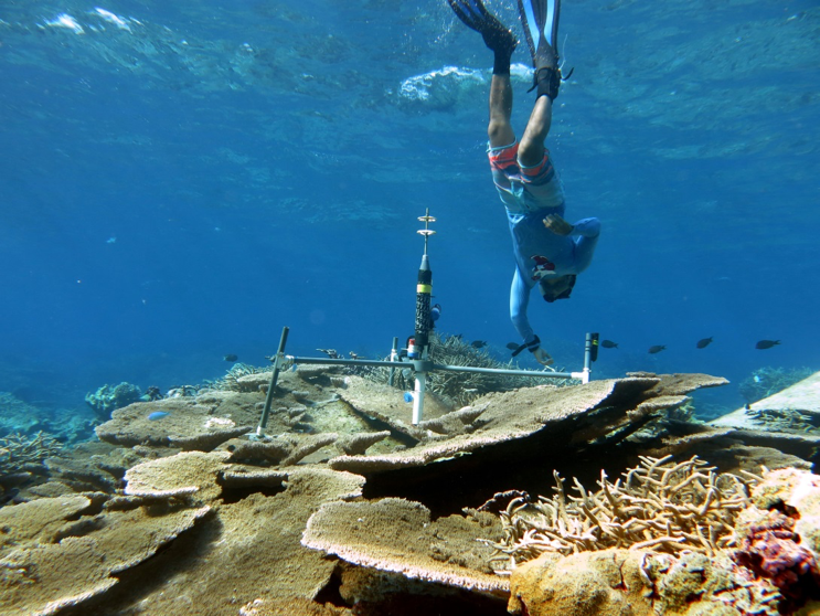
Two BEAMS were simultaneously deployed on Palmyra Atoll located approximately one km apart over vastly different benthic communities. One site was a healthy reef with approximately 70% coral cover, and the other was a degraded reef site with only 5% coral cover that was dominated by a non-calcifying invasive corallimorph Rhodactis howesii. Over the course of two weeks, BEAMS collected over 1,000 measurements of NCP and NCC from each site, yielding significantly different ratios of NCP to NCC between the two sites. These initial results suggest that BEAMS is capable of detecting different metabolic states, as well as patterns consistent with degrading reef health.
BEAMS is an exciting new autonomous tool to monitor reef health and study drivers of reef metabolism on timescales ranging from minutes to months (and potentially years). Additionally, autonomous measurement tools increase the potential for widespread and comparable observations across reefs and reef systems. Such knowledge will greatly improve our ability to predict the fate of coral reefs in a changing ocean.
Authors:
Yui Takeshita (Monterey Bay Aquarium Research Institute)