trace elements :: Ocean Carbon & Biogeochemistry

Studying marine ecosystems and biogeochemical cycles in the face of environmental change

Archive for trace elements

Ice sheets mobilize trace elements for export downstream

Posted by mmaheigan

· Thursday, January 7th, 2021

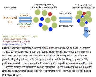
Trace elements are essential micronutrients for life in the ocean and also serve as valuable fingerprints of chemical weathering. The behaviour of trace elements in the ocean has gained interest because some of these elements are found at vanishingly low concentrations that limit ecosystem productivity. Despite delivering >2000 km³ yr^-1 of freshwater to the polar oceans, ice sheets have largely been overlooked as major trace element sources. This is partly due to a lack of data on meltwater endmember chemistry beneath and emerging from the Greenland and Antarctic ice sheets, which cover 10% of Earth’s land surface area, and partly because meltwaters were previously assumed to be dilute compared to most river waters.

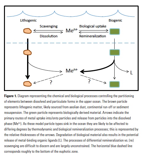
In a study published in PNAS, authors analysed the trace element composition of meltwaters from the Mercer Subglacial Lake, a hydrologically active subglacial lake >1000 m below the surface of the Antarctic Ice Sheet, and a meltwater river emerging from beneath a large outlet glacier of the Greenland Ice Sheet (Leverett Glacier). These subglacial meltwaters (i.e., water travelling along the ice-rock interface beneath an ice mass) contained much higher concentrations of trace elements than anticipated. For example, typically immobile elements like iron and aluminium were observed in the dissolved phase (<0.45 µm) at much higher concentrations than in mean river or open ocean waters (up to 20,900 nM for Fe and 69,100 nM for Al), but exhibited large size fractionation between colloidal/nanoparticulate (0.02 – 0.45 µm) and soluble (<0.02 µm) size fractions (Figure 1). Subglacial physical and biogeochemical weathering processes are thought to mobilize many of these trace elements from the bedrock and sediments beneath ice sheets and export them downstream. Antarctic subglacial meltwaters were more enriched in dissolved trace elements than Greenland Ice Sheet outflow, which is likely due to longer subglacial residence times, lack of dilution from surface meltwater inputs, and differences in underlying sediment geology.

These results indicate that ice sheet systems can mobilize large quantities of trace elements from the land to the ocean and serve as major contributors to regional elemental cycles (e.g., coastal Southern Ocean). In a warming climate with increasing ice sheet runoff, subglacial meltwaters will become an increasingly dynamic source of micronutrients to coastal oceanic ecosystems in the polar regions.

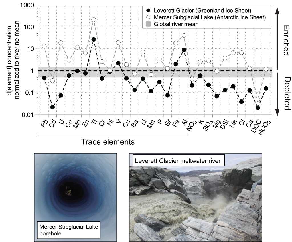
Figure caption: Leverett Glacier (Greenland Ice Sheet) and Mercer Subglacial Lake (Antarctic Ice Sheet) dissolved elemental concentrations (<0.45 µm) normalized to mean non-glacial riverine trace element concentrations (Gaillardet et al., 2014) and major element concentrations (Martin and Meybeck, 1979). Grey regions indicate ±50 % of the riverine mean. Although major elements can be significantly depleted compared to non-glacial rivers, trace elements are commonly similar to or enriched.

Authors:
Jon R. Hawkings (Florida State Univ and German Research Centre for Geosciences)
Mark L. Skidmore (Montana State Univ)
Jemma L. Wadham (Univ of Bristol, UK)
John C. Priscu (Montana State Univ)
Peter L. Morton (Florida State Univ)
Jade E. Hatton (Univ of Bristol, UK)
Christopher B. Gardner (Ohio State Univ)
Tyler J. Kohler (École Polytechnique Fédérale de Lausanne, Switzerland)
Marek Stibal (Charles University, Prague, Czech Republic)
Elizabeth A. Bagshaw (Cardiff Univ, UK)
August Steigmeyer (Montana State Univ)
Joel Barker (Univ of Minnesota)
John E. Dore (Montana State Univ)
W. Berry Lyons (Ohio State Univ)
Martyn Tranter (Univ of Bristol, UK)
Robert G. M. Spencer (Florida State Univ)
SALSA Science Team

Pumped up by the cold: Increased elemental density in polar diatoms

Posted by mmaheigan

· Monday, October 28th, 2019

Large diatoms are common in polar phytoplankton blooms, contributing significantly to food webs and carbon export, but relatively little is known about their elemental biogeochemistry. A recent study in Frontiers in Marine Science showed that the size-dependent increase in cell nutrient content for polar diatoms was similar to published values for temperate diatoms, whereas the elemental density (mass per unit volume) of polar diatoms was substantially greater for all elements measured (carbon, nitrogen, silicon and phosphorus). Furthermore, at near freezing culture temperatures, there was a positive relationship between diatom size and realized growth rates near their theoretical maximum (Figure 1). Because of the differences in elemental density between carbon and silica, these diatoms exhibited particulate C:Si ratios that are commonly interpreted as a sign of iron limitation; yet these cultures were trace metal-replete. The observed elemental composition differences suggest that it may be important for polar biogeochemical models to include different representations of diatom biogeochemistry by accounting for the functions of size and near freezing temperature.

Figure 1. Left: Cellular carbon content for polar diatoms across four orders of magnitude in biovolume compared to the same relationship for a wide range of non-polar diatoms (MD&L = Menden-Deuer & Lessard, 2000). The y-intercept is the estimate of the baseline carbon density in these polar diatoms, and is significantly higher than the literature values reviewed in MD&L (2000). Right: Growth rate of the same polar diatoms expressed as a percent of their calculated maximum growth rate at 2°C. Error bars represent the range of values observed in the experiments. Maximum growth rate was estimated by 1) applying the growth rate/biovolume relationships published by Chisholm (1992) and Edwards et al. (2012) to the observed biovolume for each culture, and 2) scaling this growth rate to 2°C growth temperature using the relationship of Eppley (1972).

Authors:
Michael Lomas (Bigelow Laboratory for Ocean Sciences)
Steven Baer (Maine Maritime Academy)
Sydney Acton (Dauphin Island Sea Lab)
Jeffrey Krause (Dauphin Island Sea Lab and University of South Alabama)

Deep ocean carbon reconstruction helps decipher a million-year-old climate mystery

Posted by mmaheigan

· Tuesday, July 23rd, 2019

Approximately one million years ago, Earth’s periodic ice ages increased in strength and duration, shifting from a 41,000-year pacing to a 100,000-year pacing, both linked to Earth’s orbital variations. The causes of this climate shift known as the mid-Pleistocene transition (MPT) have been debated for decades.

A recent study in Nature Geoscience addresses how the ocean carbon cycle contributed to the MPT by quantifying the carbon inventory of the deep Atlantic Ocean during this time. Using trace element and isotope ratios of fossil marine foraminifera, the authors demonstrate that an abrupt weakening of deep ocean overturning circulation between 950,000 and 900,000 years ago occurred alongside a pronounced increase in carbon content of the deep Atlantic Ocean. This study revealed significantly higher carbon concentrations in the deep North and South Atlantic basins during the post-MPT 100,000-year ice ages relative to the 41,000-year ice ages prior to the MPT (Figure 1).

Figure 1 caption: The last two million years of glacial cycles, with present day on left and age increasing from left to right. Orange data are from 41,000-year ice ages; blue data are from,100,000-year ice ages. (A) Glacial-interglacial cycles demonstrated in benthic oxygen isotopes (green), with warmer interglacials up and peak ice ages downward. (B) Atmospheric CO₂ from ice core measurements (gray lines) and reconstructed from boron isotopes (circles) (C), Peak ice age neodymium isotope ratios indicating strength of density-driven deep ocean circulation (squares and triangles indicate two different sediment cores). (D) Peak ice age deep ocean carbon content (squares and diamonds indicate two independent reconstructions from the same South Atlantic sediment core).

These data indicate that since 950,000 years ago, the deep Atlantic Ocean has stored an extra 50 billion tons of carbon during peak ice ages. This study hypothesizes that this extra carbon was sequestered from the atmosphere via a feedback between Antarctic ice sheet extent and the efficiency of air-sea carbon exchange in the Southern Ocean. The authors propose that intensification of ice ages one million years ago was closely linked to enhanced ocean carbon storage and resultant lowering of atmospheric CO₂ levels.

While paleoclimatologists consider the MPT to be the most recent major climate transition, the magnitude of carbon perturbation at the MPT pales in comparison to today’s human emissions. Today, humans produce 50 billion tons of carbon in only five years. Studies of the carbon cycle across past climate transitions like the MPT provide key insights on how future climate may respond to today’s carbon cycle disruption.

Authors
Jesse Farmer (LDEO Columbia University; now at Princeton University and Max Planck Institute for Chemistry)
Bärbel Hönisch, Laura Haynes, Maureen Raymo, Steven Goldstein, Maayan Yehudai, Joohee Kim (LDEO Columbia University)
Heather Ford (Queen Mary University of London)
Dick Kroon, Simon Jung, Dave Bell (University of Edinburgh)
Maria Jaume-Seguí, Leopoldo Pena (University of Barcelona)

See this related popular article and video in the Washington Post.

How fast are elements sinking in the ocean?

Posted by mmaheigan

· Tuesday, March 5th, 2019

The sinking of elements in the ocean influences many important processes such as deep ocean carbon storage and the availability of trace metals for phytoplankton. Previously, quantification of this sinking flux has been done using sediment trap deployments or tracer measurements of a particle-reactive radioisotope. Since sediment traps and each particular radioisotope each have caveats in how they quantify sinking flux, sinking particulate flux measurements, especially trace metal fluxes, are especially sparse, with relatively large uncertainties. For the first time ever, in the U.S. GEOTRACES North Atlantic campaign (GA03), four types of radioisotope data (thorium-234, polonium-210, thorium-228 and thorium-230) were measured, along with a periodic table’s worth of particulate elements that can be used to quantify sinking fluxes at locations with prior sediment trap studies, including the Ocean Flux Program (OFP), for comparison.

Sinking flux estimates of particulate organic carbon (POC) and particulate iron (pFe) derived using different methods, including the different radionuclides labelled and sediment traps from oceanic sites near Bermuda. These include the Bermuda-Atlantic Time-series site (BATS), the Ocean Flux Program site (OFP), and the Bermuda Rise (BaRFlux site). The GA03 and BaRFlux data represent observations from 2012 and 2013. The triangles and stars represent data from throughout the time-series observations of those sites.

In a new study published in Global Biogeochemical Cycles, a team of collaborators synthesized all of the radioisotope and particle composition measurements from the GA03 cruise, as well as results from a nearby study called BaRFlux, to constrain sinking fluxes of carbon and eight trace elements (P, Cd, Co, Cu, Mn, Al, Fe and thorium-232) throughout the North Atlantic Ocean. The five different methods for constraining flux (sediment traps plus the four radioisotope methods) agree encouragingly well given the independent uncertainties associated with each method. Additionally, since the four radioisotopes have a range in half-lives from days to thousands of years, the different methods can reconstruct particle fluxes throughout the water column, from the dynamic bloom-and-bust-like changes near the surface to the relatively slow, long-term sinking into the abyssal ocean. These fluxes will improve the understanding of the global budgets of carbon and trace elements. This study would not have been possible without the support of OCB and GEOTRACES who co-funded a synthesis workshop on biogeochemical cycling of trace elements at the Lamont-Doherty Earth Observatory in summer 2016.

Also see Eos highlight on this article

Authors:
Christopher T. Hayes (University of Southern Mississippi)
Erin E. Black (Woods Hole Oceanographic Institution, now at Dalhousie University)
Robert F. Anderson (Lamont-Doherty Earth Observatory of Columbia University)
Mark Baskaran (Wayne State University)
Ken O. Buesseler (Woods Hole Oceanographic Institution)
Matthew A. Charette (Woods Hole Oceanographic Institution)
Hai Cheng (Xi’an Jiaotong University and University of Minnesota)
Kirk Cochran (Stony Brook University)
Lawrence Edwards (University of Minnesota)
Patrick Fitzgerald (Stony Brook University)
Phoebe J. Lam (University of California Santa Cruz
Yanbin Lu (Earth Observatory of Singapore)
Stephanie O. Morris (Woods Hole Oceanographic institution)
Daniel C. Ohnemus (Bigelow Laboratory for Ocean Sciences, now at Skidaway Institute of Oceanography)
Frank J. Pavia (Lamont-Doherty Earth Observatory of Columbia University)
Gillian Stewart (Queens College, City University of New York)
Yi Tang (Queens College, City University of New York)

New BioGEOTRACES data sets: Connecting pieces of the microbial biogeochemical puzzle

Posted by mmaheigan

· Wednesday, December 19th, 2018

Microorganisms play a central role in the transfer of matter and energy in the marine food web. Microbes depend on micronutrients (e.g. iron, cobalt, zinc, and a host of other trace metals) to catalyze key biogeochemical reactions, and their metabolisms, in turn, directly affect the cycling, speciation, and bioavailability of these compounds. One might therefore expect that marine microbial community structure and the functions encoded within their genomes might be related to trace metal availability in the ocean. The overall productivity of marine ecosystems—i.e. the amount of carbon fixed through photosynthesis—could in turn be influenced by trace metal concentrations.

For over a decade, the international GEOTRACES program has been mapping the distribution and speciation of trace metals across vast ocean regions. Given the important relationship between trace metals and the function of marine ecosystems, biological oceanographers collaborate with GEOTRACES scientists to simultaneously probe the biotic communities at some sampling sites, allowing these biological data to be interpreted in the context of detailed chemical and physical measurements.

Figure 1. Locations and depths of samples. (a) Global map of sample locations. Single cell genomes are represented by miniaturized stacked dot-plots (each dot represents one single cell genome), with organism group indicated by color, and cells categorized as “undetermined” if robust placement within known phylogenetic groups failed due to low assembly completeness/quality or missing close references. Larger points correspond to stations on associated GEOTRACES sections where metagenomes were also collected. (b) Depth distribution of metagenome samples along each of the four GEOTRACES sections. Transect distances are calculated relative to the first station sampled in the indicated orientation. For clarity, the depth distribution of samples collected below 250 m are not shown to scale (ranging from 281–5601 m). Adapted from Berube et al. (2018) Sci. Data 5:180154 and Biller et al. (2018) Sci. Data 5:180176.

Two recent papers published in Scientific Data describes two new, large-scale biological data sets that will facilitate studies aimed at understanding how microbes and metals relate to one another. Collected on four different sets of GEOTRACES cruises (Figure 1), these papers report the public availability of hundreds of single cell genomes and microbial community metagenomes from the Pacific and Atlantic Oceans. The single cell genomes focus on the marine photosynthetic bacteria Prochlorococcus and Synechococcus and how they and other community members vary in different regions of the ocean. The metagenomic sequences provide snapshots of the entire microbial community found in each of these samples, yielding a broad overview of which microbes—and which genes, including those important for understanding nutrient cycling—are found in each sample. These two datasets are complementary and further enhanced by the wealth of chemical and physical data collected by GEOTRACES scientists on the same water samples. In particular, iron is of key interest, since it often limits primary productivity. These data sets can directly link iron availability with microbial community structure and gene content across ocean basins.

With these data, researchers can now ask questions such as how microbes have evolved in response to the availability or limitation of key nutrients and explore which organisms may be contributing to biogeochemical cycles in different parts of the global ocean. The extensive suite of chemical and physical measurements associated with these sequence data underscore their potential to reveal important relationships between trace metals and the microbial communities that drive biogeochemical cycles. These data sets also encourage cross-disciplinary collaborations and provide baseline information as society faces the challenges and uncertainties of a changing climate.

Authors:
Paul M. Berube (Massachusetts Institute of Technology)
Steven J. Biller (Massachusetts Institute of Technology; current affiliation: Wellesley College)
Sallie W. Chisholm (Massachusetts Institute of Technology)

Sinking particles as biogeochemical hubs for trace metal cycling and release

Posted by mmaheigan

· Thursday, September 14th, 2017

The extent to which the return of major and minor elements to the dissolved phase in the deep ocean (termed remineralization) is decoupled plays a major role in setting patterns of nutrient limitation in the global ocean. It is well established that major elements such as phosphorus, silicon, and carbon are released at different rates from sinking particles, with major implications for nutrient recycling. Is this also the case for trace metals?

A recent publication by Boyd et al. in Nature Geoscience provides new insights into the biotic and abiotic processes that drive remineralization of metals in the ocean. Particle composition changes rapidly with depth with both physical (disaggregation) and biogeochemical (grazing; desorption) processes leading to a marked decrease in the total surface area of the particle population. The proportion of lithogenic metals in sinking particles also appears to increase with depth, as the biogenic metals may be more labile and hence more readily removed.

Findings from GEOTRACES process studies revealed that release rates for trace elements such as iron, nickel, and zinc vary from each other. Microbes play a key role in determining the turnover rates for nutrients and trace elements. Decoupling of trace metal recycling in the surface ocean and below may result from their preferential removal by microbes to satisfy their nutritional requirements. In addition, the chemistry operating on particle surfaces plays a pivotal role in determining the specific fates of each trace metal. Teasing apart these factors will take time, as there is a complex interplay between chemical and biological processes. Improving our understanding is crucial, as these processes are not currently well represented by state-of-the-art ocean biogeochemical models.

Figure caption: Rapid changes in the characteristics of sinking particles over the upper 200 m as evidenced by: a) differential release of trace metals from sinking diatoms; b) changes in proportion of lithogenic versus biogenic materials; and c) ten-fold decrease in total particle surface area.

Authors:
Philip Boyd (IMAS, Australia)
Michael Ellwood (ANU, Australia)
Alessandro Tagliabue (Liverpool, UK)
Ben Twining (Bigelow, USA)

Relevant links:
GEOTRACES Digest: Iron Superstar

Joint workshop with GEOTRACES in August 2016: Biogeochemical Cycling of Trace Elements within the Ocean

Biogeochemical Cycling of Trace Elements Within the Ocean: A Synthesis Workshop

Posted by mmaheigan

· Sunday, September 18th, 2016

Over 100 scientists from 12 nations met at the Lamont-Doherty Earth Observatory in Palisades New York, USA, on 1 – 4 August 2016 for a synthesis workshop on the Biogeochemical Cycling of Trace Elements within the Ocean. The workshop focused on setting priorities for utilizing GEOTRACES trace element and isotope (TEI) data sets to advance scientific objectives at the interface of marine biogeochemistry and ecology, and was jointly sponsored by the GEOTRACES and OCB Programs.

Workshop activities were organized around three scientific themes:
1. Biological uptake and trace element bioavailability,
2. Abiotic cycling and scavenging, including particulate and dissolved speciation, and
3. Export, recycling and regeneration

Following a series of plenary talks designed to stimulate discussion on these topics, participants spent the remainder of the workshop in smaller group discussions to identify knowledge gaps and develop ideas for synthesis activities and products that combine GEOTRACES TEI data with other biogeochemical and biological data sets.

Tentative activities and products include:
• estimating bioavailability of iron (Fe)
• testing hypothesis for Fe and light co-limitation in the deep chlorophyll maxima;
• exploring Redfieldian concepts using GEOTRACES data and ocean models;
• calculating community trace metal demand vs. supply;
• developing a synthesis paper on existing methods and current state of knowledge on ligand composition and cycling;
• comparing radionuclide-based tracer methods for estimating downward flux of carbon, nutrients and trace metals;
• combining TEI distributions with AOU and preformed TEI concentrations to differentiate biotic (e.g., respiration) and abiotic (e.g., scavenging, physical transport) removal processes;
• estimating elemental scavenging using partition coefficients (Kd);
• combining particulate TEI and beam transmission data to develop algorithms for particle distributions that affect TEI scavenging; and
• developing synthesis paper on TEIs in nepheloid layers.

To learn more about and/or contribute to these activities, please contact Heather Benway (OCB) or Bob Anderson (LDEO). For more information, visit the workshop website or view the plenary presentations.

Trace metal uptake and remineralization and their impact on upper ocean stoichiometry

Posted by mmaheigan

· Wednesday, July 6th, 2016

1. Stoichiometry of metals in the ocean

The close relationship between the stoichiometry of nutrients dissolved in the upper ocean and the planktonic organisms that grow in these waters has long been recognized (1, 2). The stoichiometry of 106 C:16 N:1 P first summarized by Redfield has become a fundamental concept of marine biogeochemistry, with numerous studies using the ratio as a benchmark to assess ecosystem function. Decades after the work of Redfield, with the implementation of trace metal-clean techniques, oceanographers produced the first meaningful measurements of dissolved trace metals in the open ocean (3-5), and they found that many of the bioactive metals such as Fe, Zn, Ni, Cu and Cd are also depleted in surface waters and enriched at depth, similar to the macronutrients. Such nutrient-like behavior supported not only a growing understanding of the physiological roles that these metals play in phytoplankton physiology (6), but it also indicated that biological uptake and sub-surface remineralization were important processes for controlling the distributions of these bioactive metals in the ocean. Thus, the biogeochemical behavior of the micronutrient metals is in many ways analogous to that of the macronutrients N, P and Si.

In the open ocean far from coastal and shelf influences, dissolved concentrations of bioactive metals increase with depth at relatively consistent ratios to macronutrients (5), and these metal:nutrient remineralization ratios have been used to approximate the composition of sinking biogenic material and euphotic zone phytoplankton (7, 8). These ‘extended Redfield ratios’ have been compared to average compositions of marine phytoplankton species grown in culture (9-12), and the general agreement between these approaches further supports the importance of biological uptake and subsequent remineralization of trace metals in the upper ocean as key processes impacting trace metal geochemistry. Average metal:nutrient stoichiometries for phytoplankton have also been compared to dissolved stoichiometries in the ambient water, and relationships between these fractions have been used to estimate nutrient limitation and deficiency in the ocean (13). Thus, there is significant interest in controls on upper ocean metal stoichiometries, as well as the relationships between cellular/biological, particulate and dissolved fractions.

Analogous to macronutrients, there are also relationships between metal stoichiometries in phytoplankton and those in deeper waters of the ocean. Departures from these relationships are likely to provide insights into the internal biogeochemical cycling of metals in the ocean. Morel and Hudson (7) noted differences in the extended stoichiometries of plankton and the water column and concluded that they must reflect the relative efficiency of remineralization of the elements, as well as the propensity of elements to be scavenged onto sinking particles in the sub-surface ocean. Similarly, the rapid remineralization of trace metals from sinking plankton was addressed in seminal work by Collier and Edmond (14). Using carefully collected data on surface plankton material, and with more computational rigor than (7), they compared surface particle stoichiometries to deep water dissolved stoichiometries and calculated the relative remineralization of plankton-associated elements in sinking biogenic material. They noted significant differences among the behaviors of biogenic metals such as Cd, Ni and Fe due to their scavenging and remineralization behaviors. More recently, Morel (15) mused about these processes and their relationships to cellular biochemistry and evolution of phytoplankton physiology and ocean biogeochemistry.

Through the GEOTRACES program, the data to test and extend these early, relatively simple box models and stoichiometric comparisons are now available. Metal concentrations and stoichiometries for phytoplankton, bulk and size-fractionated particulate material, and co-located dissolved species have been measured in the North Atlantic and South Pacific Oceans thus far. Combined with data for non-bioactive metals such as Ti and Th, these data also provide the opportunity to discern the behavior and contributions of lithogenic vs. biogenic matter, as well as the processes of remineralization and scavenging.

2. Processes affecting dissolved and particulate stoichiometries of trace metals

Vertical profiles of dissolved macronutrients show characteristic depletion at the surface and enrichment at depth due to remineralization, and dissolved micronutrients often show the same behavior. However, the internal cycling of metals in the ocean is expected to differ from that of macronutrients for a few salient reasons. Some metals such as Fe are significantly less soluble than macronutrients and are prone to abiotic adsorption onto particulate surfaces (16). This process is driven by thermodynamics, and the accompanying process of desorption also occurs; the net observed process is typically called ‘scavenging’ (Fig. 1). Scavenging in the deep ocean causes concentrations of less soluble metals such as Fe and Al to decrease along the path of thermohaline circulation, in contrast to macronutrients and more soluble metals that may mimic macronutrient behavior such as Cd and Zn (17). In the absence of significant lateral nutrient inputs, the balance of scavenging and remineralization will influence the resulting vertical profiles of dissolved elements (18).

Another key difference between macronutrients and metals is the importance of abiotic particulate fractions such as lithogenic (e.g., aeolian dust and sediment) and authigenic (e.g., Fe- and Mn-oxyhydroxide) phases. While biogenic phases are almost universally produced at the surface and remineralized with depth, abiotic phases can exhibit very different and dynamic internal cycles (19). Dust events, lateral transport and poorly constrained scavenging processes can both deliver and remove specific metals alongside biological processes. Lithogenic phases are generally denser and more refractory than biogenic particles and detritus and are thought to sink more rapidly and remineralize more slowly and at greater depth (Fig. 1; 20). Lithogenic particles may also (re)scavenge metals differently than biogenic material. Efforts to examine these processes in sinking material have been extremely limited to date, with only a few studies examining metals in trace metal-clean sediment traps (21, 22). However, recently published datasets from the GEOTRACES program are shedding new light on the multiple facets of metal partitioning and how they affect subsurface remineralization and scavenging.

A comparison of metal:phosphorus ratios in the upper ocean illuminates some of these processes. Figure 2 displays Cd:P, Fe:P, Co:P and Ni:P ratios in particles in the upper 100m, 100-300m, and 300-1,000m of the water column in the middle of the North Atlantic basin. Particulate material is sub-divided into ratios for phytoplankton cells and non-lithogenic particles (corrected for lithogenic minerals using Ti; 19). Also plotted are dissolved remineralization ratios (that is, the slope of a linear regression between the dissolved metal and phosphate) for these upper ocean depth ranges. The close coupling of Cd and P biogeochemistry has long been recognized (4), and indeed we observe very close agreement (within a factor of about 2) between dissolved Cd:P remineralization and Cd:P in surface ocean particles, as well subsurface particles. Clearly these elements are remineralizing from sinking particles at similar rates. Such comparisons of particulate and dissolved constituents need to carefully consider the different residence times of these fractions and the likelihood for lateral inputs. Here, we have chosen to focus on stations from the mid-North Atlantic gyre, where the upper 700m of the water column consists primarily of a single water mass (23).

In contrast, the remineralization of Fe and P are quickly decoupled in the water column (Fig. 2). Between 100 and 300m, typically the depth of most rapid regeneration of sinking organic material, labile particulate Fe:P has more than doubled from that in surface waters, and the Fe:P ratio of remineralized dissolved elements (0.98 mmol/mol) is more than 10-fold below that of the labile material that is sinking into these waters. Looking deeper into the water column, Fe and P continue to decouple in labile (i.e., non-lithogenic) particulates, with Fe:P of 300-1,000m particles increasing 10-fold and the dissolved remineralization ratio being nearly 1,000-fold lower (0.35 mmol/mol). Additionally, organic ligands play an important role in stabilizing dissolved Fe (24), so dissolved Fe and P ratios may be further decoupled by biological processes impacting the production and fate of these ligands (20).

A strength of GEOTRACES datasets is their wide coverage of the periodic table, and additional insights can be gained from looking at the behaviors of other bioactive trace metals that are also incorporated into sinking biogenic material. Co:P ratios in particles and remineralized dissolved fractions in the water column follow the same trend as Fe, but the decoupling of Co and P is much more subtle than with Fe, presumably due to differences in ligand coordination and Co co-oxidation with Mn (25, 26). Dissolved Co:P remineralization ratios at 100-300m generally match those found in phytoplankton and drop only 3-fold below 300m. Similarly, labile particulate Co:P ratios don’t change between 0-100m and 100-300m, also indicating that Co and P remineralize in tandem in the upper 300m. Below 300m, labile particulate Co:P increases approximately 3-fold (in contrast with Fe:P, which increases 12-fold), and this depth effect matches the effect in dissolved remineralization ratios. Thus, even though Fe and Co are considered hybrid metals that display both biological uptake and scavenging, there are clear differences in the behaviors of these metals. Nickel provides yet another perspective on the coupling of metals and P. Dissolved remineralization ratios in both subsurface depth ranges closely resemble surface ocean labile particles, supporting the biological coupling of Ni and P (5). However, residual labile particulate Ni:P increases 2- to 4-fold in successive depth ranges, indicating that remineralization is rather decoupled. Given that Ni seems to be associated with both organic material and opal frustules in diatoms (27), it may be that Ni and P are remineralized from particulate organic matter in tandem, but some Ni remains associated with sinking biogenic silica in the ocean.

3. Additional tools to explore and differentiate remineralization processes

The GEOTRACES program has welcomed the application of new analytical approaches that further enable us to study the cycling of metals in the ocean. Spectroscopy and quantitative imaging methods using synchrotron radiation have become more common in the past decade (28), and these allow us to analytically distinguish the behaviors of different fractions of particle assemblages. During the FeCycle II project, a GEOTRACES process study, the fate of Fe was tracked during a spring diatom bloom (29). Diatom cells from the dominant bloom species (Asterionellopsis glacialis) were collected in surface waters and from trace-metal clean sediment traps at 100m and 200m in the 48h following the decline of the bloom. Synchrotron x-ray fluorescence (SXRF) analyses of individual cells showed that constituent elements were lost from sinking cells at notably different rates (Fig. 3). Phosphorus was rapidly released from sinking cells, with mean P quotas decreasing 55% and 73% from surface values by 100m and 200m, respectively (30). However, only 25% of cellular Fe was lost from cells sinking through the upper 200m, while 61% of cellular Ni was remineralized. This supports the story told by the bulk biogeochemical data from the North Atlantic: Ni is remineralized largely to a similar degree as P, while Fe is lost more slowly from sinking biogenic material.

Application of microanalytical techniques such as SXRF can be combined with bulk approaches to further advance understanding of subsurface metal remineralization and cycling. In FeCycle II, Fe:P of sinking A. glacialis cells increased, on average, only 2.3-fold in the upper 200m, while Fe:P in bulk particulate matter increased more than 13-fold (30). This indicates that the behavior of sinking cells was not representative of the full particle assemblage. Iron and P were likely more completely decoupled in sinking fecal pellets and detrital material (which appears to have contributed significantly to the particulate Fe pool during FeCycle II; 31) than in intact sinking cells. Further application of this approach will allow us to not only distinguish between the behavior of biogenic and lithogenic fractions (Fig. 1), but potentially also between detrital particles. By considering metals such as Mn that are prone to oxidation and scavenging in the subsurface ocean (32, 33), it may also be possible to separate abiotic scavenging from net biological remineralization (Fig. 1). Additionally, 2D (and potentially 3D) mapping of elements within cells and particles also provides information about the spatial and potentially chemical associations of elements with particles (30, 34).

The GEOTRACES program is generating unprecedented data, both in terms of quality and quantity, regarding the cycling of bioactive trace metals in the ocean. Syntheses of these data, and integration of insights from novel microanalytical tools, as well as transcriptomic and proteomic approaches, are resulting in substantial advances in our understanding of metal biogeochemistry. No longer are we limited to a few painstakingly collected dissolved metal profiles. There is now painstakingly collected full-depth coverage of most ocean basins, including in many cases dissolved and particulate fractions of nearly all biogenic elements, enabling testing of early hypotheses about trace metal cycling and parameterization of these processes into next-generation ocean biogeochemical models.

Authors

Benjamin S. Twining, Daniel C. Ohnemus, Renee L. Torrie (Bigelow Laboratory for Ocean Sciences)

Acknowledgments

This work was funded by NSF grant OCE-1232814 to BST. RLT was funded by NSF REU grant 1460861 to Bigelow Laboratory for Ocean Sciences.

References

1. A. C. Redfield, in James Johnstone Memorial Volume, R. J. Daniel, Ed. (Liverpool University Press, 1934), pp. 176-192.
2. A. C. Redfield, Amer. Scientist 46, 205-221 (1958).
3. E. A. Boyle, J. M. Edmond, Nature 253, 107-109 (1975).
4. E. A. Boyle, F. Sclater, J. M. Edmond, Nature 263, 42-44 (1976).
5. K. W. Bruland, Earth Plan. Sci. Lett. 47, 176-198 (1980).
6. J. R. R. Frausto da Silva, R. J. P. Williams, The Biological Chemistry of the Elements: the inorganic chemistry of life. (Oxford University Press, Oxford, ed. 2nd, 2001), pp. 575.
7. F. M. M. Morel, R. J. M. Hudson, in Chemical Processes in Lakes, W. Stumm, Ed. (John Wiley & Sons, New York, 1985), pp. 251-281.
8. K. W. Bruland, J. R. Donat, D. A. Hutchins, Limnol. Oceanogr. 36, 1555-1577 (1991).
9. T. Y. Ho et al., J. Phycol. 39, 1145-1159 (2003).
10. W. G. Sunda, Marine Chem. 57, 169-172 (1997).
11. W. G. Sunda, S. A. Huntsman, Limnol. Oceanogr. 40, 132-137 (1995).
12. W. G. Sunda, S. A. Huntsman, Limnol. Oceanogr. 40, 1404-1417 (1995).
13. C. M. Moore et al., Nature Geosci. 6, 701-710 (2013).
14. R. Collier, J. Edmond, Prog. Oceanogr. 13, 113-199 (1984).
15. F. M. M. Morel, Geobiol. 6, 318-324 (2008).
16. M. Whitfield, D. R. Turner, in Aquatic Surface Chemistry: Chemical Processes at the Particle-Water Interface, W. Stumm, Ed. (John Wiley & Sons, Inc., 1987), pp. 457-493.
17. K. W. Bruland, M. C. Lohan, in The Oceans and Marine Geochemistry: Treatise on Geochemistry, H. Elderfield, Ed. (Elsevier, Oxford, 2003), pp. 23-47.
18. P. W. Boyd, M. J. Ellwood, Nature Geosci. 3, 675-682 (2010).
19. D. C. Ohnemus, P. J. Lam, Cycling of lithogenic marine particles in the US GEOTRACES North Atlantic Transect. Deep-Sea Res. II 116, 282-302 (2015).
20. P. W. Boyd et al., Limnol. Oceanogr. 55, 1271-1288 (2010).
21. R. D. Frew et al., Glob. Biogeochem. Cycles 20, GB1S93, doi:10.1029/2005GB002558 (2006).
22. C. H. Lamborg, K. O. Buesseler, P. J. Lam, Deep-Sea Res. II 55, 1564-1577 (2008).
23. W. J. Jenkins et al., Deep-Sea Res. II 116, 6-20 (2015).
24. M. Gledhill, K. N. Buck, Frontiers Microbiol. 3, doi: 10.3389/fmicb.2012.00069 (2012).
25. J. W. Moffett, J. Ho, Geochim. Cosmochim. Acta 60, 3415-3424 (1996).
26. A. E. Noble et al., Limnol. Oceanogr. 57, 989-1010 (2012).
27. B. S. Twining et al., Glob. Biogeochem. Cycles 26, GB4001, doi:4010.1029/2011GB004233 (2012).
28. P. J. Lam et al., Prog. Oceanogr. 133, 32-42 (2015).
29. P. W. Boyd et al., Geophys. Res. Lett. 39, doi:10.1029/2012GL053448 (2012).
30. B. S. Twining et al., Limnol. Oceanogr. 59, 689-704 (2014).
31. A. L. King et al., Biogeosci. 9, 667-687 (2012).
32. J. P. Cowen, K. W. Bruland, Deep-Sea Res. 32, 253-272 (1985).
33. D. C. Ohnemus et al., Limnol. Oceanogr. In press (2016).
34. J. Nuester, S. Vogt, B. S. Twining, J. Phycol. 48, 626-634 (2012). 35. B. S. Twining et al., Prog. Oceanogr. 137, 261-283 (2015).
36. M. Hatta et al., Deep-Sea Res. II 2015, 117-129 (2015).
37. S. Roshan, J. Wu, Glob. Biogeochem. Cycles 29, 2082-2094 (2015).
38. E. Mawji et al. Marine Chem. 177, 1-8 (2015).

Marine particles: Distribution, composition, and role in scavenging of TEIs

Posted by mmaheigan

· Sunday, July 3rd, 2016

GEOTRACES and particles in the ocean

GEOTRACES is an international program to study the global marine biogeochemical cycles of trace elements and their isotopes (TEIs). The program’s guiding mission is to “identify processes and quantify fluxes that control the distributions of key TEIs in the ocean” (1).

Particles represent a key parameter for the GEOTRACES program because of their role as sources, sinks, and in the internal cycling of so many TEIs (1, 2). Particles in the ocean fall into two classes: 1. Those that have sources external to the system such as lithogenic material carried by atmospheric transport, river, or lateral transport from continental margin sediments; and 2. those that are produced internally in the system, primarily by biological production, but also by authigenic mineral precipitation (2).

External particle sources such as mineral dust deposition and sediment resuspension act as sources of dissolved TEIs when they partially dissolve in seawater. Conversely, dissolved TEIs are removed by active biological uptake or passive adsorption onto particles surfaces, followed by particle removal by aggregation and sinking. Indeed, the biological and abiotic interactions of dissolved TEIs with particles determine the residence time of a dissolved TEI.

In most open ocean basins away from ocean floor boundaries, external sources of particles are dwarfed by the much greater biological production and destruction of particles. Particle cycling in most open ocean basins is thus dominated by the biological pump, the processes by which suspended particles are produced by photosynthesis in the euphotic zone at the surface, and are then abiotically or biologically aggregated into larger particles that can sink into the abyss (3).

As particulate organic carbon (POC) cycles through processes such as aggregation, disaggregation, remineralization, and sinking (collectively referred to here as particle dynamics), other particle phases are swept along for the ride, including other major components such as biologically precipitated minerals (especially CaCO₃and opal), as well as lithogenic and authigenic particles, and scavenged TEIs adsorbed to the surfaces of other particles (Fig. 1).

In this article, I will briefly review the role of particle composition on the scavenging of TEIs.

Scavenging: A two-step removal process

Most adsorption of TEIs likely occurs onto small, suspended particles, which are usually more abundant, have more available surface area, and have a longer residence time in the water column than large, sinking particles. For TEIs to be removed from the water column, the suspended particles must then be aggregated into larger, sinking particles. There are thus two distinct steps for the removal of a dissolved TEI by scavenging: 1) adsorption onto suspended particle surfaces, followed by 2) removal via the aggregation of suspended particles onto larger particles that sink out of the water column. Fig. 1 shows a very simple schematic illustrating these basic processes. The adsorption step is governed by the affinity of a TEI for a particular particle surface, and the removal step is governed by the particle dynamics that package suspended particles into large, sinking aggregates, and are the focus of studies of the biological pump. The removal of TEIs by scavenging thus intimately links one of OCB’s scientific goals, the understanding of the biological carbon pump, to GEOTRACES’s mission to identify processes and quantify fluxes that control the distributions of key TEIs in the ocean.

Particle concentration and composition: horizontal and vertical variations

Particles collected in the ocean are a heterogeneous mixture of biogenic, lithogenic, and authigenic (precipitated in-situ) components. The relative proportions of these different components vary geographically and with depth. Fig. 2 shows the distribution of total particle concentration from GA03, the U.S. GEOTRACES North Atlantic Zonal Transect cruise in 2010/2011, as well as the changing composition of small (<51 mm) particles at three stations along the transect (4). Particle concentrations are highest at the surface and at the margins, where biological production is highest. It is clear that particulate organic matter (POM) dominates particle composition in the upper 100 m, making up more than 70% of the suspended particle mass at all three stations. The balance in the upper 100 m is mostly made of other biogenic components such as CaCO₃and opal, with a small contribution from lithogenic particles directly under the Saharan dust plume. At all stations, the inorganic components (everything except for POM) become relatively more important with depth as POM is remineralized. In the eastern half of the basin, lithogenic particles make up the largest fraction of particle mass, accounting for >50% of particle mass below 1500 m. In the western half of the basin, further from the Saharan dust source, lithogenic particles are not as important, and CaCO₃makes up the largest fraction (~50%) of particle mass between 500 – 3000 m. A special case is found in a station over the Mid-Atlantic Ridge, where iron oxyhydroxides from the hydrothermal plume make up ~50% of the particle mass. Iron and manganese oxyhydroxides are rarely dominant components of particle mass, except in special situations such as hydrothermal plumes, but may exert a particularly large influence on TEI adsorption (5, 6 ).

Studies suggest that particle composition may affect both the affinity of dissolved TEIs for adsorbing onto particle surfaces (2), and the vertical flux of particles from the water column (7-9). Horizontal and vertical changes in particle composition thus allow us to test hypotheses of the importance of particle composition on both steps in the scavenging of TEIs.

Effect of particle composition on adsorption of TEIs

The affinity of TEIs to particles has typically been characterized by a partition coefficient, Kd, which is calculated empirically as:

Prior to the GEOTRACES program, the effect of particle composition on TEI adsorption affinity had been studied in the field using sediments and sinking particles collected in sediment traps. The affinity of trace metals to marine sediments of different compositions varied: Some trace metals (Cs, Be, Sn, and Fe) had a higher affinity to sediments dominated by aluminosilicate clay minerals, and others (Ba, Cd, Zn, Mn, and Co) had a higher affinity to sediments enriched in Mn oxyhydroxides (10). In the water column, correlations between the partition coefficient of ²³⁰Th and particle composition in sediment trap particles from around the world have variously implied that the scavenging efficiency of ²³⁰Th is controlled by CaCO₃(11, 12), lithogenic material (13, 14), and/or Mn oxyhydroxides (15). Studies that span strong opal gradients across the Polar Front in the Southern Ocean show higher partition coefficients for ²³¹Pa scavenging in areas of high opal content (11, 16). ²³¹Pa is generally not as particle-reactive as ²³⁰Th in the open ocean, but is often removed with equal efficiency as ²³⁰Th in near-margin areas (e.g., 17), presumably because opal is more important in margin settings. The Arctic, on the other hand, displays the opposite ²³⁰Th/²³¹Pa removal signal, with ²³¹Pa removal less efficient relative to ²³⁰Th at the margins compared to the open ocean (18).

Since TEIs adsorb primarily onto suspended particles rather than sinking particles, studying the correlations between partition coefficients and suspended particles may resolve some of the discrepancies observed in the sediment trap studies (c.f., 2).

The GEOTRACES GA03 North Atlantic Zonal Transect has provided the first opportunity to investigate the correlation between partition coefficients of various TEIs and the particle composition of suspended particles in the ocean. Thus far, this has been done for ²³⁰Th and ²³¹Pa partition coefficients, with Mn and Fe oxyhydroxides emerging as key controlling phases and opal having no controlling effect (5). The North Atlantic is very opal-poor (Fig. 2), so particles collected from more diatom-rich regions are needed to examine the potential of opal as a controlling phase. Other studies are underway to study the particle affinities of Hg (19), Po (20), and Pb (6) on this same North Atlantic transect. Subsequent U.S. GEOTRACES sections (GP16—Eastern Tropical South Pacific Zonal Transect and GN01—Western Arctic) will also have full ocean depth size-fractionated particle concentration and composition, allowing us to examine samples from different biogeochemical provinces, and hopefully expanding the range of particle compositions.

TEIs as tracers of scavenging rates and particle dynamics

The unprecedented data sets from GEOTRACES are also allowing us to estimate adsorption and desorption rate constants (Fig. 1) from inverse modeling of the observations of dissolved and particulate TEIs and particle concentrations (19, 21, 22). This gives us a kinetic view of the scavenging process to complement the empirically-derived partition coefficients, which are often viewed as representing equilibrium constants. Applying inverse modeling approaches to observations of the distributions of size-fractionated particles and particulate TEIs can also allow us to estimate rates of particle remineralization, aggregation, disaggregation, and sinking (21, 23). This approach requires only that a conceptual model relating the suspended and sinking particle size fractions be applied to observations of particle mass and particulate TEIs, and does not require knowledge about which specific physical or biological processes are responsible for particle transformations. For example, Fig. 1 illustrates a simple conceptual model in which a pool of suspended particles can be lost to the dissolved phase through remineralization, or by aggregation into sinking particles; conversely, sinking particles can sink, or can be disaggregated back into suspended particles. By assuming that particulate TEIs are simply part of the overall particle pool (e.g., a coating on organic particles in the case of radiogenic TEIs such as ²³⁰Th or as part of a lithogenic particle in the case of a TEI such as Ti) and thus are subject to the same rates of particle transformations as the major phases such as POC, we can apply the same conceptual model to observations of particle mass and to observations of particulate TEI to better constrain the rates of these transformations (23). As some of these rates such as aggregation and disaggregation are notoriously difficult to measure directly, these inverse approaches offer a way forward to quantify these important processes.

Particle composition and the biological pump

In addition to its effect on scavenging efficiency, particle composition has also been implicated as an important factor in the strength and efficiency of the biological pump. Several meta-analyses of global deep (>1000 m) sediment trap data showed strong correlations between POC flux and mineral flux (7-9), leading to the development of the “ballast hypothesis.” The mechanisms to explain the correlations, which are still being debated (24, 25), range from mineral protection of POC (8), mineral contribution to particle excess density (7), scavenging of mineral particles by POC (26), and minerals as proxies for particle packaging, POC lability, and ecosystem structure (9, 27-29).

Although the GA03 dataset is based on size-fractionated particle samples collected by in-situ filtration rather than sinking particles collected by sediment traps, we can nonetheless examine whether there is a correlation between POC and ballast minerals in small or large particle size fractions. We found that POC concentration in large (>51 mm) particles was not consistently correlated with any of the potential ballast minerals CaCO3, opal, and lithogenic particles (4).The lack of strong correlations within this regional dataset is consistent with the idea that ballast mineral correlations with POC may only emerge in global datasets that combine different biogeochemical provinces (25).

Outlook

The GEOTRACES program is not only rapidly expanding global observations of dissolved TEIs, but it is also the latest major program to systematically sample particle distributions since JGOFS and GEOSECS (2). These particle measurements are not only helping us understand the processes controlling TEI distributions, but the TEI measurements can also be used as tracers for quantifying key processes of particle cycling. Both GEOTRACES and OCB can benefit from the insights gained in each program.

Author

Phoebe J. Lam (Department of Ocean Sciences, University of California, Santa Cruz)

References

1. GEOTRACES, Scientific Committee on Oceanic Research, Ed. (Baltimore, Maryland, 2006).
2. C. Jeandel et al., Progress in Oceanography 133, 6 (4//, 2015).
3. C. L. De La Rocha, in Treatise on Geochemistry, H. Elderfield, K. K. Turekian, Eds. (Elsevier, 2003), vol. 6: The Oceans and Marine Geochemistry, pp. 83-111.
4. P. J. Lam et al., Deep Sea Research Part II: Topical Studies in Oceanography 116, 303 (6//, 2015).
5. C. T. Hayes et al., Marine Chemistry 170, 49 (3/20/, 2015).
6. E. A. Boyle et al., paper presented at the 2016 Ocean Sciences Meeting, New Orleans, LA, USA, 2016.
7. C. Klaas, D. E. Archer, Global Biogeochemical Cycles 16, 1116 (Dec 5, 2002).
8. R. A. Armstrong et al., Deep-Sea Research Part II-Topical Studies in Oceanography 49, 219 (2002).
9. R. François et al., Global Biogeochemical Cycles 16, (Oct-Nov, 2002).
10 . L. S. Balistrieri, J. W. Murray, Geochimica Et Cosmochimica Acta 48, 921 (1984).
11. Z. Chase et al., Earth and Planetary Science Letters 204, 215 (Nov 30, 2002).
12. Z. Chase et al., Deep-Sea Research Part II-Topical Studies in Oceanography 50, 739 (2003).
13. S. D. Luo, T. L. Ku, Earth and Planetary Science Letters 220, 201 (Mar, 2004).
14. M. Roy-Barman et al., Earth and Planetary Science Letters 286, 526 (2009).
15. M. Roy-Barman et al., Earth and Planetary Science Letters 240, 681 (2005).
16. H. J. Walter et al., Earth and Planetary Science Letters 149, 85 (1997).
17. R. F. Anderson, M. P. Bacon, P. G. Brewer, Earth and Planetary Science Letters 66, 73 (1983).
18. H. N. Edmonds et al., Earth and Planetary Science Letters 227, 155 (Oct, 2004).
19. C. H. Lamborg et al., Philos T R Soc A, (accepted).
20. Y. Tang et al., paper presented at the 2016 Ocean Sciences Meeting, New Orleans, LA, USA, 2016.
21. O. Marchal, P. J. Lam, Geochimica Et Cosmochimica Acta 90, 126 (2012).
22. P. Lerner et al., Deep Sea Research Part I: Oceanographic Research Papers 113, 57 (7//, 2016).
23. P. J. Lam, O. Marchal, Annual Review of Marine Science 7, 159 (2015).

24. P. Boyd, T. Trull, Progress in Oceanography 72, 276 (2007).
25. J. D. Wilson, S. Barker et al., Global Biogeochemical Cycles 26, GB4011 (2012).
26. U. Passow, Geochemistry Geophysics Geosystems 5, (Apr 6, 2004).
27. P. J. Lam et al., Global Biogeochem. Cycles 25, GB3009 (2011).
28. S. A. Henson et al., Global Biogeochem. Cycles 26, GB1028 (2012).
29. S. Z. Rosengard et al., Biogeosciences 12, 3953 (2015).
30. D. C. Ohnemus, P. J. Lam, Deep Sea Research Part II: Topical Studies in Oceanography 116, 283 (6//, 2015).

Using GEOTRACES data to appraise iron cycling as represented within global ocean models

Posted by mmaheigan

· Thursday, June 23rd, 2016

We rely on global ocean models to predict how climate change might affect the evolution of ocean productivity, acidification, and deoxygenation (1). Such platforms are also used to test hypotheses regarding the controls on ocean biogeochemical cycling and to understand past change (both on historical and geologic timescales). Ocean biogeochemistry models began with relatively simple formulations of a carbon export flux that involved restoring to observed phosphate distributions, but have more recently evolved into complex multi-element representations of the ocean. In line with our understanding that the trace micronutrient iron (Fe) limits phytoplankton productivity over large areas of the world ocean (2), most global models that aim to project future change also explicitly represent the Fe cycle.

Datasets regarding the major limiting nutrients (nitrate, phosphate, and silicate) have been available as gridded ‘climatologies’ since the early 1990s (3). This has greatly facilitated the development and evaluation of modelled distributions over the past two decades. However, over this period there has been little comprehensive evaluation of how different models represent the ocean Fe cycle. Over recent years, there has been a marked increase in the availability of iron measurements in the ocean (4), largely driven by the international GEOTRACES effort to conduct full depth, basin-scale surveys. This led us to initiate the first-ever attempt to critically compare a range of global ocean iron models against the largest global datasets, as well as against the newly emerging ocean section data (5).

The Fe Model Intercomparison Project (FeMIP) sought to be as inclusive as possible in this first step and therefore did not seek to standardize the underlying ocean circulation or external inputs. Instead, we simply asked each of the thirteen models to provide their best representation of dissolved iron in three dimensions at monthly resolution. We then compared these models against each other, a global iron database of over 20,000 observations and against five unique basin-scale sections from the GEOTRACES intermediate data product 2014 (IDP2014) (6).

Firstly, it is apparent that even when the underlying iron cycles of the different models are evaluated, a substantial degree of inter-model discord exists. The total iron input varies from around 2 to 200 Gmol yr-1 across the thirteen models (Fig. 1a). Even for ‘well known’ sources like atmospheric deposition, the inter-model variability is around an order of magnitude. On the other hand, the average concentrations of dissolved Fe between the models is much less variable and ranges from 0.35 to 0.81 nmol L-1 (Fig. 1b), or an average of 0.58±0.14 nmol L-1. This apparent constancy reflects an initial view of the ocean Fe cycle in which interior Fe concentrations were held at a quasi-constant value of 0.6 nmol L-1 assuming a constant concentration of Fe-binding ligands (7). Thus the FeMIP models are balancing widely varying Fe input fluxes against relatively constant overall Fe concentrations by tuning the Fe scavenging rate, which is a crucial but poorly known parameter. This results in residence times for Fe that range from <5 to >500 years across the FeMIP models (Fig 1c). This difference is important, as it represents substantial inter-model deviation concerning the timescales over which the different models respond to a perturbation in Fe supply.

When compared statistically against the global dataset, similar levels of variability arise. Some models display correlation coefficients of >0.5, whereas others are slightly anti-correlated. When the FeMIP models are compared against the five GEOTRACES sections, it becomes apparent that those models that represent the newly emerging features of the iron cycle perform much better. For instance, having Fe scavenging rates that vary in space and time, including variable Fe:carbon (C) stoichiometry, multiple Fe sources, and representing ligand concentrations in a dynamic manner, all act to improve the representation of different observed features in the models. Importantly, the IDP2014 provided the opportunity to demonstrate that the issues at hand were specific to Fe, since the models could represent the observed distributions of major nutrients with a much greater degree of skill (5).

The next stage of FeMIP will be a deeper comparison of the processes themselves. Of particular interest is whether GEOTRACES datasets can provide broader assessments of the rates of Fe scavenging – e.g., using other particle-reactive, non-biological tracers such as thorium (8, 9). Equally, the emerging database of GEOTRACES process studies provides an important opportunity to appraise the way different models represent biological iron cycling and in particular, the often-observed importance of recycled and remineralized sources of Fe (10, 11). Finally, the new GEOTRACES intermediate data product 2017 will also facilitate further evaluation of models, providing new section data from the Atlantic, Pacific and Arctic Oceans.

Author

Alessandro Tagliabue (Dept. of Earth, Ocean and Ecological Sciences, School of Environmental Sciences, University of Liverpool)

References

1. L. Bopp et al., Biogeosci. 10(10), 6225-6245, doi:10.5194/bg-10-6225-2013 (2013).
2. C. M. Moore et al., Nature Geosci., doi:10.1038/ngeo1765 (2013).
3. S. Levitus et al., Prog. Oceanogr. 31(3), 245-273, doi:10.1016/0079-6611(93)90003-v (1993).
4. A. Tagliabue et al., Biogeosci. 9(6), 2333-2349, doi:10.5194/bg-9-2333-2012 (2012).
5. A. Tagliabue, A. et al., Glob. Biogeochem. Cycles, doi:10.1002/2015gb005289 (2016).
6. E. Mawji et al., Marine Chem. 177, 1-8. doi:10.1016/j. marchem.2015.04.005 (2015).
7. K. S. Johnson, R. M. Gordon, K. H. Coale, Marine Chem. 57(3-4), 137-161, doi:10.1016/s0304-4203(97)00043-1 (1997).
8. C. T. Hayes et al., Geochim. Cosmochim. Acta 169, 1-16, doi:10.1016/j.gca.2015.07.019 (2015).
9. N. Rogan et al., Geophys. Res. Lett. 43(6), 2732-2740. doi:10.1002/2016gl067905 (2016).
10. P. W. Boyd et al., Glob. Biogeochem. Cycles 29(7), 1028-1043, doi:10.1002/2014gb005014 (2015).
11. R. F. Strzepek et al., Glob. Biogeochem. Cycles 19(4), GB4S26, doi:10.1029/2005gb002490 (2005).

Funding for the Ocean Carbon & Biogeochemistry Project Office is provided by the National Science Foundation (NSF) and the National Aeronautics and Space Administration (NASA). The OCB Project Office is housed at the Woods Hole Oceanographic Institution.

Archive for trace elements

1. Stoichiometry of metals in the ocean

2. Processes affecting dissolved and particulate stoichiometries of trace metals

3. Additional tools to explore and differentiate remineralization processes

Authors

Acknowledgments

References

GEOTRACES and particles in the ocean

Scavenging: A two-step removal process

Particle concentration and composition: horizontal and vertical variations

Effect of particle composition on adsorption of TEIs

TEIs as tracers of scavenging rates and particle dynamics

Particle composition and the biological pump

Outlook

Author

References

Author

References

Filter by Keyword